HINT 18A: Find the variance in offspring number and substitute into the formula on page 419. However, that formula is for a diploid population of 2N genes: For a haploid population of N genes, replace 2N by N.
HINT 18B: Find the mean fitness of this allele.
HINT 18C: Write the probability of loss, Q, as a sum over the possibilities of having 0, 1, or 2 offspring (see Chapter 28).
HINT 18D: Think about whether any mutations are likely to have occurred on the lineages that connect two genes to their common ancestor (see p. 426).
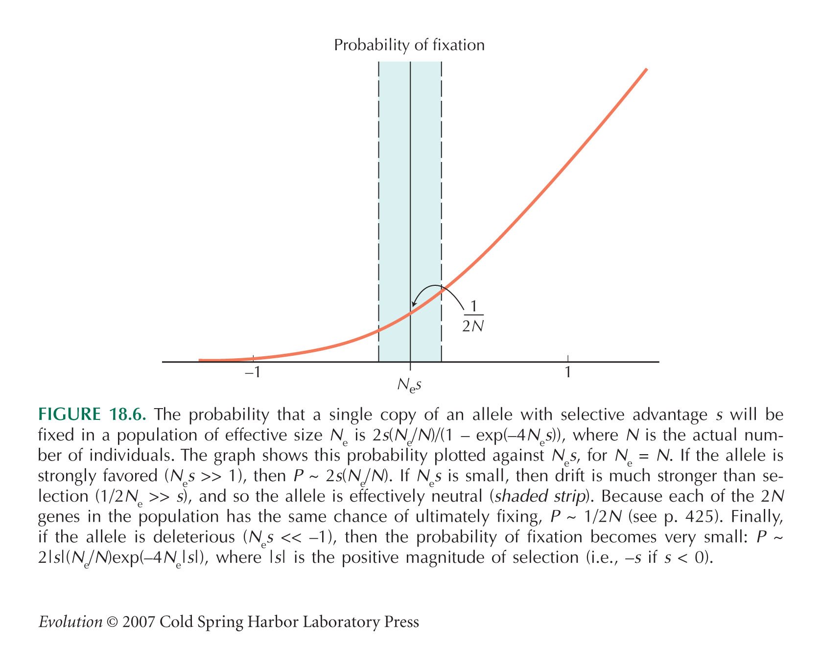
HINT 18E: See Figure 18.6.
HINT 18F: At equilibrium, the rate of shifts from GUU must equal the rate of shifts to GUU.
HINT 18G: We are dealing with deleterious alleles, and so the s in the formula of Figure 18.6 is negative. Changing s to –s gives 2s(Ne/N)(exp(4Nes) – 1).
HINT 18H: Recall that the selection gradient is defined as the increase in relative fitness per increase in trait value. Thus, we can measure it relative to the standard deviation of environmental variation, ![]() . For example, the trait might be measured in grams, in which case β would have dimensions of per gram.
. For example, the trait might be measured in grams, in which case β would have dimensions of per gram.
HINT 18I: Start by thinking about the contribution of a single diploid locus and then sum over all the loci.
HINT 18J: See answer to Problem 17.12.
HINT 18K: Think about the number of favorable mutations produced and the proportion that are fixed.
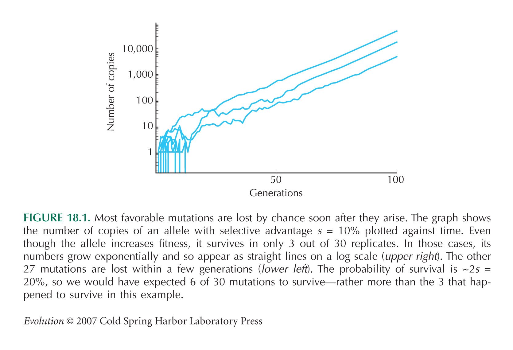
HINT 18L: See Figure 18.1.
HINT 18M: A normal distribution with variance σ2t at time t is given by density, (1/(2πσ2t)) exp(–x2/2σ2t), where x is the distance from the point of origin. Note that this does not have a square root in the denominator, because it describes spread in two dimensions, not one dimension.
HINT 18N: See pp. 496–497.
HINT 18O: Think about the spread of the allele through a two-dimensional space.
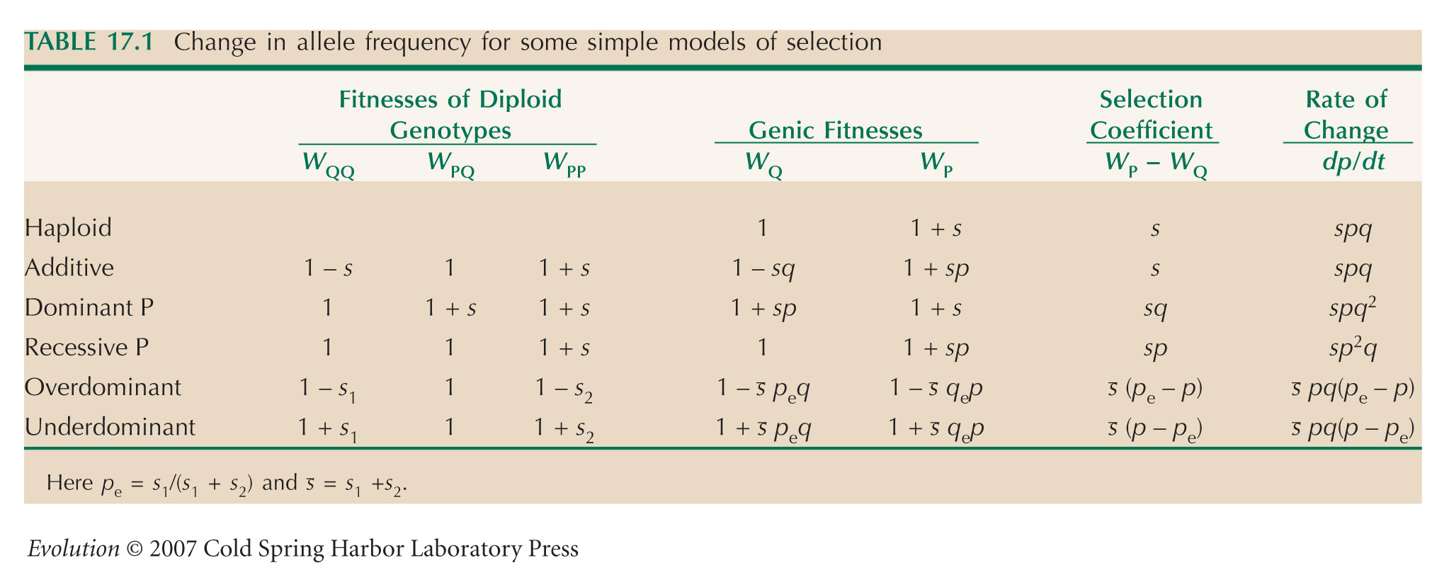
HINT 18P: The equation representing diffusion is explained in Chapter 28, and the equation for the effects of underdominance is given in Table 17.1.
HINT 18Q: Differentiating p with respect to x and rearranging shows that dp/dx = apq. Then, differentiate again.
HINT 18R: Expect the same amount of polymorphism in each deme; look for an equilibrium with p1 = q2, p2 = q1.
HINT 18S: Set p1 = ![]() + ε1, p2 =
+ ε1, p2 = ![]() + ε2, where
+ ε2, where ![]() ,
, ![]() are the equilibrium allele frequencies. Ignore small terms such as ε12 (see Chapter 28).
are the equilibrium allele frequencies. Ignore small terms such as ε12 (see Chapter 28).
HINT 18T: You cannot assume Hardy–Weinberg proportions because this incompatibility system has evolved to ensure nonrandom mating: Homozygotes cannot be produced.
HINT 18U: Think about invasion of each allele from low frequency.
HINT 18V: Plot the rate of increase of P from low frequency against α and similarly for the rate of increase of Q from low frequency.
HINT 18W: First, work out the initial frequency of allele P within patch A, and within B.
HINT 18X: Assume that mating is random.
HINT 18Y: See Box 18.2.
HINT 18Z: You can assume that the population mean is at the optimum, zopt = ![]() , and that the allele is rare.
, and that the allele is rare.
HINT 18AA: exp(–y) ~ 1 – y for small y.
HINT 18BB: The total mutation rate over the diploid genome is U = 2nμ.
HINT 18CC: Assume that mutations affect these traits in the same way.
HINT 18DD: We must balance the increased numbers of alleles due to mutation against the loss due to selection against heterozygotes and against homozygotes.
HINT 18EE: Show that this has the form exp(–BF) and estimate B.
HINT 18FF: To find the equilibrium allele frequency, balance the increased numbers of alleles due to mutation against the loss due to selection against heterozygotes and against homozygotes.
HINT 18GG: Because both homozygotes have the same fitness, the allele frequencies will stay equal regardless of how much inbreeding there is.
HINT 18HH: Calculate the average decrease in fitness of an individual and multiply by the number of genes.