Boundary Conditions for the Diffusion Equation

We can understand what happens at extreme allele frequencies (i.e., p = 0, 1) by thinking of the flux of probability (i.e., the net rate at which populations change their allele frequency). The diffusion equation (Eq. 36) for the allele frequency, p, can be written as

where

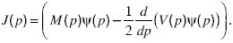
The quantity J(p) is called the probability flux. Imagine very many populations that follow the distribution of allele frequencies ψ(p). In a small time δt, some will increase their allele frequency from below a threshold, p, to above it, whereas others will decrease. The net proportion of populations that evolve from below p to above p is just Jδt. At equilibrium, this flux is zero; solving J = 0 gives the equilibrium distribution.

Suppose that a fraction A₀ of populations have very low allele frequency, with p < p₀ << 1, and a fraction A₁ are almost fixed at very high allele frequency, with q < q₁ << 1. Then, the rate of increase of A₀ must equal the rate at which populations fall below p₀ ~ 0:

Similarly, the rate of increase of A₁ must equal the rate at which populations rise above the threshold p₁, which is close to 1:

To understand these boundary conditions, think of a population evolving under mutation, selection, and random drift. The expected rate of change of allele frequency is M(p) = spq + µq – νp, where the rate of mutation from Q to P is µ and from P to Q is ν. The variance of allele frequency fluctuations is V(p) = pq/2N_e. Near the boundaries, selection is negligible relative to mutation and drift: For example, near p = 0, M ~ µ, and V ~ p/2N_e. Thus,

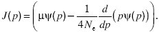
This has the solution ψ = C₀ p^{4N_eµ – 1}. Thus, if the numbers of mutations entering the population are high enough (4N_eµ > 1), there is a negligible chance of being at very low frequency. However, if 4N_eµ < 1, the distribution becomes very large at the boundaries, implying that there is a high probability that one of the alleles will be lost. At equilibrium, J = 0, and so A₀ stays constant. However, if the distribution is out of equilibrium, we can work out how the fractions fixed near 0 and 1 change through time.