NOTE 19M: This is a t-test with 9 degrees of freedom.
NOTE 19N: If the selection coefficient really were s = 1.2%, then in some experiments the null hypothesis (s = 0) would be rejected, and in some it would not be. The fraction of cases in which the null hypothesis would be rejected, given that s = 1.2%, is known as the statistical power. This gives a better measure of the chance of detecting a given selection coefficient.
NOTE 19O: This formula is for neutral alleles, whereas here there is some selection. However, selection is fairly weak, and so the error is not too great.
NOTE 19P: In principle, this could be caused by a changing selection coefficient on the F allele itself: strongly negative, then weakly positive, and then approaching zero. However, conditions are supposedly constant, and frequency-dependent selection cannot account for the changing direction of selection: Allele frequency falls rapidly when in the range 0.4–0.1 in the first few generations, but then rises again through the same range of allele frequencies between generations 10 and 40.
NOTE 19Q: We can also look at the variability in the data. The variance of allele frequency around the equilibrium in the last 50 generations is 0.0033 (i.e., a standard deviation of 0.058). The variance expected from sampling 100 diploid individuals, or 200 genes, is pq/2N = 0.39 × 0.41/200 = 0.00080, which is higher than this. Therefore, there is no evidence of any extra variation due to drift: The population has a large effective size.
NOTE 19R: The mixing of different populations and selection against heterozygotes is expected to lead to a deficit of heterozygotes. However, there is no clear indication of a deficit of D/d in these data.
NOTE 19S: Better estimates would take into account the mode of inheritance: At the first two loci, one phenotype is due to a recessive allele, whereas at the third, the heterozygote is intermediate. See Mallet et al. (1990).
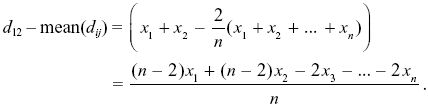
NOTE 19T: Following Kimura, the variance is estimated as the sum of squares of deviations, divided by n = 6. Often, n – 1 = 5 is used in the denominator, which will give a somewhat larger variance.
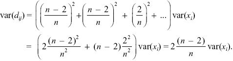
NOTE 19U: To see the relation between var(dij) and var(xi), consider the deviation from the mean:
The expectation of the square of this deviation is found by summing the expectations of the squares of each term, because the xi are independent of each other (i.e., E[xixj] = 0, E[xi2] = var(xi)). So,
NOTE 19V: This could be estimated separately for each gene, and the separate αs averaged. These αs would be quite unreliable, however, because a low value of Dn in the denominator (e.g., at AP50 or hem) would produce a very negative α.
NOTE 19W: We have ignored the initial random establishment of the favorable allele. Given that it will be fixed, its expected frequency is higher than this simple deterministic prediction by a factor 2s; in effect, the initial frequency is 1/4Ns, rather than 1/2N. So, a better prediction would be (1/s)loge(4Ns). However, this makes little difference to the estimate because the dependence is via a logarithm. See Problem 18.5.
NOTE 19X: Indeed, the estimated total mutation rate is based on the assumption that the rate of molecular evolution is equal to the mutation rate, which assumes neutrality; this rate of the molecular clock is, however, similar to direct estimates, which implies that most mutations cannot be significantly deleterious.
NOTE 19Y: In fact, a nucleotide site can have only one of four possible bases, so the maximum nucleotide diversity is π = 3/4.
NOTE 19Z: This problem is similar to Problem 18.2, which uses calculations of fixation probability to find the extent of codon usage bias.
NOTE 19AA: This calculation makes the simplifying assumption that the population is almost always fixed. Then, recombination is irrelevant, because only one substitution is in progress at any one time. In fact, if there is polymorphism, Stephan and Kirby (1993) and Stephan (1996) show that the rate of evolution is greater when the paired sites are tightly linked.
NOTE 19BB: The measure of association uP – uQ is equal to D/pq, where D is the coefficient of linkage disequilibrium. (To see this, recall that the frequency of uP within BP genomes is (pu + D)/p = u + D/p and similarly uQ = u = D/q.)
NOTE 19CC: Maynard and Haigh (1974) were originally motivated by the need to explain why random drift seems to occur even in very large populations, so that genetic diversity is not extremely high. This point of view has been extended recently by Gillespie (2000a,b). Gillespie terms the cumulative effect of hitch-hiking “genetic draft,” in contrast to “random drift.” Although the rate of increase of variance in allele frequency is the same, for the same effective population size, the two processes are otherwise very different, and can in principle be distinguished by comparing patterns of variation (see pp. 536–538).
NOTE 19DD: The exact result can be found using the methods of Box 28.2. We have du/dt = (dp/dt)(1 – u0) exp(–ct). Now, we know that pt/qt = (1/2N) exp(st), and so exp(–ct) = (2N pt/qt)–c/s, and
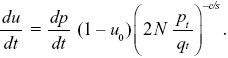
Treating u as a function of p (as in Box 28.2), we have
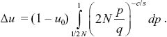
This does not have an explicit solution, but for 2N large is very close to (2N)–c/s, as given by the simple argument above.