 |
|
|
|
|
Evolution Chapter 16 Answers
|
Answer 16.1
|
| i) |
In each generation, a fraction m = 10/100 = 0.1 come from outside. The new allele frequency is therefore pt = mpS+(1 – m)pt–1, where the allele frequency in the source is pS = 1. It is easier to work with the frequency of the native allele, qt = 1 – pt, since qS = 0, and so qt = (1 – m)qt–1. After 20 generations, therefore, p20 = 1 – q20 = 1 – 0.920 = 0.878.
|
| ii) |
Similarly, p20 = 1 – 0.9920 = 0.182.
|
| iii) |
The rate of immigration, m, now varies from generation to generation: it is m = 10/20 for one generation in ten, and 10/1000 otherwise. Hence,

Gene flow mostly occurs during the brief times when the native population is small. NOTE 16C
|
|
Answer 16.2
|
| i) |
The equilibrium will be a linear cline. Using the same method as that in Box 16.1, we know that allele frequency changes according to
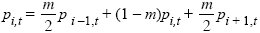
where pi – 1,t is the ith deme in the line. So, at equilibrium, we must have
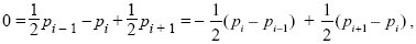
which means that the difference in allele frequency between each pair must stay the same. Because the ends are fixed at p1 = 0, p6 = 1, we have p2 = 0.2, p3 = 0.4, p4 = 0.6, p5 = 0.8. This is independent of the rate of gene flow, m.
|
| ii) |
The same argument as above holds for the demes on either side. At the center, we must have
p3,t = 0.06 p2,t + (1 – 0.06 – 0.01)p3,t + 0.01p4,t ,
so that
0 = –0.06 (p3,t – p2,t) + 0.01(p4,t – p3,t).
Thus, a reduction in gene flow by a factor of 6 makes the gradient in allele frequency six times steeper (i.e., (p4,t – p3,t) = 6(p3,t – p2,t) = 6d, say). So, there are four intervals of size d and one of size 6d. These sum to 1, and so d = 0.1. The solution is that p2 = 0.1, p3 = 0.2, p4 = 0.8, p5 = 0.9.
|
|
Answer 16.3
|
| i) |
The rate of diffusion is the variance in distance between parent and offspring. m = 0.5 move ±100 meters, and the other half do not move. Therefore, σ2 = (1/2)(100 meters)2 per generation = 5,000 m2 per generation.
|
| ii) |
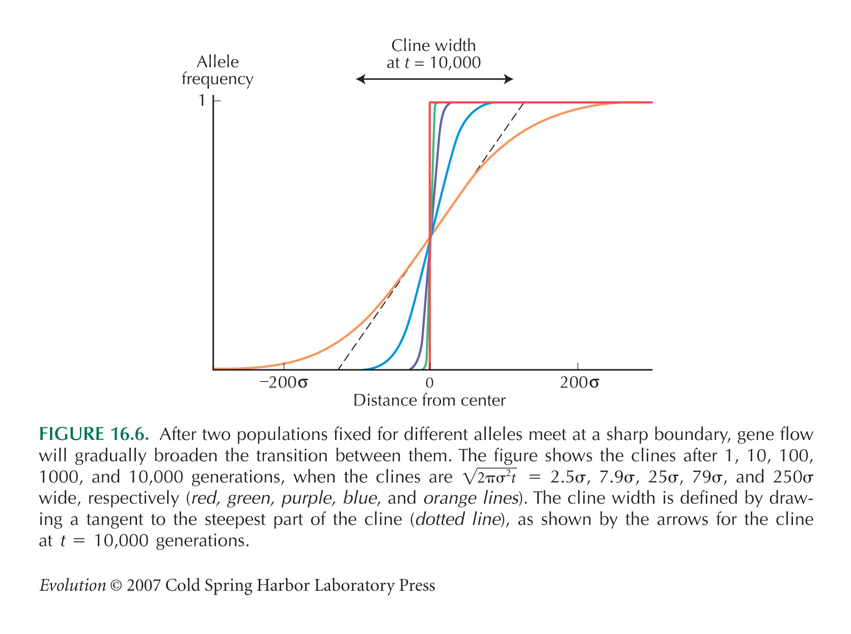
With neutral mixing, cline width after t generations is  (see Fig. 16.6). After 20 generations, this is 793 meters. The diffusion approximation, ignoring the fixed endpoints, is very accurate up to 20 generations (see Fig. P16.2). (see Fig. 16.6). After 20 generations, this is 793 meters. The diffusion approximation, ignoring the fixed endpoints, is very accurate up to 20 generations (see Fig. P16.2).
|
| iii) |
Ultimately, the cline will settle to a linear form, with width 20 × 100 m = 2 km.
|
|
Answer 16.4
|
| i) |
The mean allele frequency is 0.3, and the variance is 0.0444. Therefore, FST = var(p)/ = 0.212. = 0.212.
|
| ii) |
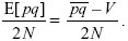
The observed variance in allele frequency will be increased by the sampling variance, which is /2n for a sample of n diploid individuals from a population with actual allele frequencies p,q. So, we expect the observed variance to be FST + E[pq]/2n, where var(p) = FST is the true variance in the actual allele frequencies. Because E[pq] = – var(p) = (1 – FST, we have an observed variance of (FST + (1 – FST)/2n). This leads to a revised estimate of FST = 0.170. (It would be a good approximation just to subtract the scaled sampling error, 1/2n = 0.05, from the estimate in i).)
|
| iii) |
Assuming conservative migration—so that gene flow does not directly alter allele frequencies—the effective size of the population as a whole is inflated by a factor 1/(1 – FST) = 1.205. However, fluctuations in population size will tend to reduce the overall Ne.
|
|
Answer 16.5
|
| i) |
From Box 16.2, 1/(1 + 4Nm). The appropriate migration rate is the average of that in males and females, (mM + mF)/2 = 0.075, because an autosomal gene spends half its time in males and half in females. Thus, FST = 0.143.
|
| ii) |
Now, the number of copies of the gene is N/2 rather than 2N, and migration is through males only. Therefore, FST = 1/(1 + NmM) = 0.333.
|
| iii) |
From Box 15.2, the effective population size for an X-linked gene is
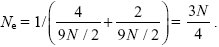
An X-linked gene spends 2/3 of its time in females and 1/3 in males, and so m = (mM/3 + 2mF/3). Thus, FST = 1/[1 + N(mM + 2mF)] = 0.2.
|
| iv) |
Following ii), but replacing males by females, FST = 1/(1 + NmF) = 0.5.
|
|
Answer 16.6
|
| i) |
The measure QST = var( )/(var() + 2VA) is expected to equal FST, on the assumption that both allozyme frequencies and the trait mean are in a balance between gene flow and random drift. Also, h2 = 0.3 = VA/VP. Therefore, var() = 0.106VP, corresponding to a standard deviation of 0.326 phenotypic standard deviations. )/(var() + 2VA) is expected to equal FST, on the assumption that both allozyme frequencies and the trait mean are in a balance between gene flow and random drift. Also, h2 = 0.3 = VA/VP. Therefore, var() = 0.106VP, corresponding to a standard deviation of 0.326 phenotypic standard deviations.
|
|
Answer 16.7
|
| i) |
Every deme traces its ancestry back through a single deme. There is no mixing, and so demes must fix at 0 or 1. Overall, a fraction q of demes is fixed at 0 and p at 1. There are no heterozygotes (E[2pq] = 0), and var(p) = , so that FST = 1.
|
| ii) |
Extinctions and recolonizations occur at a rate λn. Whenever one occurs, the new deme has frequency 0 or 1 with probability q or p. If it is 0, then the overall mean allele frequency has decreased by –p/n, whereas if it is 1, the mean has increased by + q/n. The variance of this change is q(–p/n)2 + p(–q/n)2 = pq/n2. Therefore, the rate of increase in variance of allele frequency is λpq/n. Defining this as 1/2NE, we have NE = n/λ. The faster the rate of extinction and recolonization, the faster the rate of drift, and the smaller the overall effective size.
|
| iii) |
The effect of extinction and recolonization is now quite different. If empty patches are colonized from the population as a whole, they will immediately return to the overall average allele frequency, p. Thus, extinction and recolonization now increase diversity within demes and reduce differences between them. Conversely, random drift at a rate 1/2Ne will reduce diversity within demes, and increase variation between them.
In a small time interval δt, λnδt demes will return to the overall average. Thus, differences in allele frequency will decrease by a factor (1 – λnδt), and the variance V of these differences will decrease by a factor (1 – λnδt)2 ~ 1 – 2λnδt. The decrease in variance per unit time is therefore –2λnV; this is balanced by random drift that increases V by
The net change in variance is
so that at equilibrium
|
|
Answer 16.8
|
| i) |
Provided gene flow is conservative (i.e., provided it does not change allele frequencies directly), then for any population structure, the mean coalescence time for two genes from the same deme is TW = 2nNe (see p. 449). Assuming infinite-sites mutation, we therefore expect π = 2μTW = 4nNeμ. Hence, nNe = 200,000.
|
| ii) |
(assuming that there are a large number of demes so that  ~ TB). (See p. 449.) ~ TB). (See p. 449.)
|
|
Answer 16.9
|
| i) |
Assuming Hardy–Weinberg proportions, the frequencies of the recessive sd and cr alleles are estimated as the square root of the sd/sd and cr/cr homozygotes. The frequency of the d allele is estimated directly, as half the D/d heterozygote frequency plus the d/d homozygote frequency. So, psd = 0.512, pcr = 0.476, pd = 0.518. Because the population is formed by mixing populations fixed for different alleles and because each locus is under similar selection against unusual patterns, these allele frequencies are similar.
|
| ii) |
The frequency of the double-recessive homozygote (sd/sd cr/cr say) is expected to be the square of the frequency of the double-recessive gamete (psd cr2, say). Subtracting the frequency expected at linkage equilibrium gives an estimate of the coefficient of linkage disequilibrium (D = psd cr – psdpcr, say). Thus, Dsd cr ~ 0.0453, Dcr d ~ 0.0623, and Dsd d ~ 0.0623.
|
| iii) |
The average D is 0.0566, which can be equated to the approximation σ2/(rw2), with r = 1/2 for unlinked loci, and w = 1 km. Hence, σ2 ~ 2.8 km2 per generation, a standard deviation of σ ~ 1.7 km. (See Mallet et al. [1990] for a detailed analysis.)
|
|
Answer 16.10
|
| i) |
There are 66 red alleles among 2 × 25 × 35 genes, and so the average allele frequency is p = 0.0377. The chance that an individual has no “red” alleles among 50 genes (2 copies at each of 25 loci) is therefore q50 = 0.962350 = 0.146, and the expected number in the zero class is 35 × 0.962350 = 5.12. The number with one red allele is 50pq49, the number with 2 is (50 × 49/2)p2q48, and so on, following a binomial distribution.
The individual with six red alleles is unlikely to have arisen by chance in a panmictic population, and the individual with ten “red” alleles is vanishingly unlikely.
|
| ii) |
The F1 has 25 heterozygous loci, the first generation backcross (Bx1) has 12.5 on average, and so on. Thus, the individual in class 10 is most likely to be a first-generation Bx1, and the individual with 6 is most likely to be a Bx2. However, the actual number of introgressed alleles varies widely, according to a binomial distribution, so these inferences are uncertain.
|
| iii) |
Of 35 deer, 2 are hybrids, most likely one Bx1 and one Bx2. Later backcrosses would be undetectable against the background of randomly combining alleles. Because hybrids could be detected over three generations (as F1, Bx1, or Bx2), we can estimate the rate at which F1s are produced as 2/(35 × 3) ~ 0.020 per generation. Because only half the genes of an F1 are from red, this corresponds to m = 0.01 per generation.
|
| iv) |
Assuming one-way immigration (the simplest assumption), then following the first problem, we expect allele frequency to be 1 – 0.9925 = 0.22. In fact, it is much lower. This may be because the species have met more recently than 25 generations or have only just begun to hybridize, because they overlap in a limited area, or because selection acts against introgressing alleles, or simply because by chance, there is more introgression than average in this sample. (See Goodman et al. [1999] for a full analysis.)
|
|
|
|


