 |
|
|
|
|
Evolution Chapter 14 Answers
|
Answer 14.1
|
| i) |
The mean fruit weight of the backcross population is 5.30 g, and its s.d. is 2.58 g (see Fig. P14.5). The data do not fit well to a normal curve: There are too few small fruits (<–1 s.d.) and too many large ones (>1 s.d.).
|
| ii) |
The mean is 5.27 g and the s.d. is 2.58 g. Therefore, a fruit with zero weight would be at –5.27/2.58 = –2.04 s.d., Reading from the graph of the cumulative normal distribution (Fig. P14.5, lower left), the probability of a fruit with weight less than zero would be about 0.02. The normal distribution cannot apply to data that have a definite lower bound.
|
| iii) |
The variance of fruit weight in the backcross is (2.58 g)2 = 6.66 g2. This consists of the genotypic variance plus the environmental variance. Now, because the F1 is genetically homogeneous (all individuals are heterozygous for alleles that differ between the two strains), the variance in the F1 is entirely environmental. If we assume that F1 and backcross plants have the same environmental variance, then we see that the genotypic variance in the backcross population is 6.66 – 0.71 = 5.95 g2, and the heritability is 5.95/6.66 = 0.89. NOTE 14B
|
| iv) |
Log transformed data are much closer to normal (Fig. P14.6).
|
| v) |
In the backcross, the mean log(fruit weight) is 0.68 and the variance of log(fruit weight) is 0.042 (using logarithms to base 10). Therefore, using the same argument as before, the heritability is 0.39. The large difference between heritabilities illustrates the basic point that variance components and heritabilities depend strongly on the scale of measurement. In this example, a log scale seems more natural, because then fruit weight itself must always be positive and because the distributions are closer to normal. However, choice of scale is essentially arbitrary.
|
|
Answer 14.2
Figure P14.7 shows plots of mortality against log(dose) (P1, red; P2, blue; F1, purple; F2, green). The horizontal lines are at mortality 0.025, 0.16, 0.50, 0.84, 0.975, which correspond to –2, –1, 0, 1, 2 s.d. Curves are drawn by eye.
|
| i) |
Based on where the curves cross the horizontal lines, the means and s.d. are
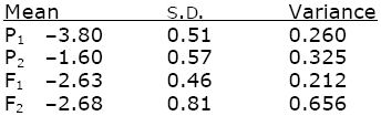
(For example, the mean of P1 is where the red curve crosses the 0.50 line, at –380. This curve crosses the line at 0.16 at –4.31, corresponding to –1 s.d.; hence 1 s.d. is –3.80 – (–4.31) = 0.5; the variance is 0.512 = 0.260.) The scale is log(dose) to the base 10.
|
| ii) |
Assuming that the F1 variance is entirely nongenetic and that this environmental variance is the same as that in the F2, we estimate Ve = 0.212, Vg = 0.656 – 0.212 = 0.444, and so h2 = Vg/(Vg + Ve) = 0.68.
|
|
Answer 14.3
|
| i) |
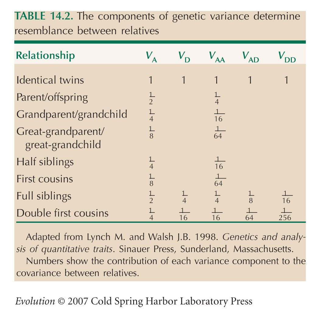
The covariance between father and son is predicted to be one-half the additive genetic variance (Table 14.2, line 2; we can ignore higher-order components such as VAA that represent epistasis). Thus, we estimate VA = 2 × 3.84 = 7.68 inches2. This is slightly greater than the variance of sons’ height (7.54 inches2), but slight differences are expected from random sampling. We estimate that all the variance in height is inherited: h2 = 1.
|
| ii) |
The covariance with mothers’ height is slightly lower; a similar calculation gives VA = 2 × 3.23 = 6.46 and h2 = 0.86. The difference might be because of sampling error. It could also be that because females are shorter on average, the effects of genes on females’ height is on average smaller. (For this reason, it might be more appropriate to do the analysis on a logarithmic scale.)
|
| iii) |
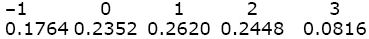
The correlation coefficient is defined as cov(x, y)/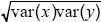 = 1.84/ = 1.84/ = 0.29. This correlation reflects a tendency for people of similar height to marry; such assortative mating is commonly found. The effect is to increase the covariance between parent and offspring, because the genes that the offspring inherits from one parent will tend to have an effect similar to those inherited from the other parent. Thus, the heritability is lower than estimated in i) and ii). NOTE 14C = 0.29. This correlation reflects a tendency for people of similar height to marry; such assortative mating is commonly found. The effect is to increase the covariance between parent and offspring, because the genes that the offspring inherits from one parent will tend to have an effect similar to those inherited from the other parent. Thus, the heritability is lower than estimated in i) and ii). NOTE 14C
|
| iv) |
If variation is entirely additive, we expect the covariance between brothers to be the same as that between parent and offspring (Table 14.2). However, dominance variance contributes to the similarity between brothers but not to that between parent and offspring. In this example, the covariance between brothers is slightly lower than that between fathers and sons. Thus, there is no evidence that dominance contributes to variance in height. NOTE 14D
|
|
Answer 14.4
|
| i), ii) |
Write the genotypic values as 1, 3, 9. The corresponding genotype frequencies, assuming Hardy–Weinberg proportions, are 0.82: 2 × 0.8 × 0.2: 0.22 = 0.64:0.32:0.04. The mean is therefore 0.64 + 3 × 0.32 + 9 × 0.04 = 1.96, and the genotypic variance is Vg = 0.64(1 – 1.96)2 + 0.32 × (3 – 1.96)2 + 0.04(9–1.96)2 = 2.92. The average excess of the two alleles is (0.8 × 1 + 0.2 × 3, 0.8 × 3 + 0.2 × 9) – 1.96 = (–0.56, 2.24) and the breeding values are therefore (–2 × 0.56, –0.56 + 2.24, 2 × 2.24) = (–1.12, 1.68, 4.48) and the additive variance is Va = 0.64(–1.12)2 + 0.32 × (1.68)2 + 0.04(4.48)2 = 2.51. The dominance deviation is the difference between the deviation of the genotypic value from the mean and the breeding value: (1 – 1.96 – (–1.12), 3 – 1.96 – 1.68, 9 – 1.96 – 4.48) = (0.16, –0.64, 2.56). The dominance variance is Vd = 0.64(0.16)2 + 0.32 × (–0.64)2 + 0.04(2.56)2 = 0.41. Necessarily, Va + Vd = Vg.
|
| iii) |
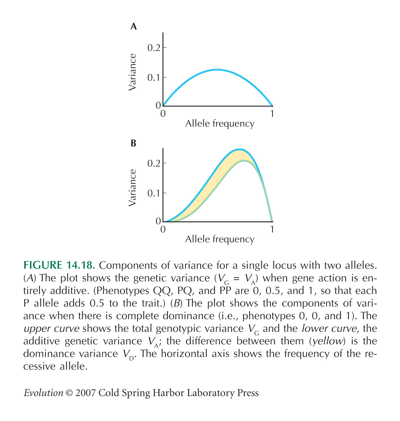
A similar calculation for allele frequencies 0.2:0.8 gives Vg = 9.06, Va = 8.65, Vd = 0.41. A larger fraction of the variation is now additive: As we saw in Figure 14.18, the relative magnitudes of the variance components change with allele frequency. Here, allele P is almost recessive (giving a large effect when homozygous), and so the dominance variance makes up a larger fraction of the total when this allele is rare.
|
| iv) |
Working with logarithms to base 10, the trait is now additive, with genotypic values 0, 0.477, 0.954. For allele frequencies 0.8:0.2, the mean is 0.32 × 0.477 + 0.04 × 0.954 = 0.191; the breeding values are just equal to the deviations of genotypic values from the mean (–0.191, 0.286, 0.763), and the additive genetic variance is Va = 0.073 and makes up the entire genotypic variance. As we saw in Problem 14.1, the relative sizes of the variance components depend on the scale on which the trait is measured. NOTE 14E
|
|
Answer 14.5
|
| i) |
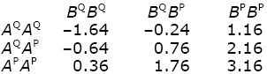
The genotype frequencies at each locus are obtained from the Hardy–Weinberg formula, assuming random mating (Box 1.1). Thus, AQAQ, AQAP, APAP are at frequencies 0.62:2 × 0.6 × 0.4:0.42 = 0.36:0.48: 0.16. Similarly, BQBQ, BQBP, BPBP are at 0.49:0.42:0.09. If there is no association between the alleles (i.e., if they are in linkage equilibrium; p. 432), then the two-locus genotype frequencies can be found by multiplying together the frequencies at each locus as follows:
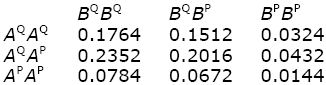
The genotypic values are found by summing these genotype frequencies. For example, AQAPBQBP and AQAPBPBP have value 2, and their combined frequency is 0.2016 + 0.0432 = 0.2448. Thus,
The mean is –1 × 0.1764 + ... + 3 × 0.0816 = 0.82. The genotypic variance is the average of the squared deviation of the genotypic value from the mean: Vg = (–1 – 0.82)2 × 0.1764 + ... + (3 – 0.82)2 × 0.0816 = 1.4796.
|
| ii) |
Because the effects of each gene add up, we can consider them separately. Genotypes AQAQ, AQAP, APAP have values –1, 0, 1. An AQ allele finds itself with AQ with probability 0.6, in which case it has value –1, and with AP with probability 0.4, in which case it has value 0. The average value of AQ is therefore –0.6, and similarly, the average for AP is 0.4. The overall mean, averaging over these two alleles, is (–0.6) × 0.6 + 0.4 × 0.4 = –0.20. Therefore, the average excess for the two alleles AQ, AP is (–0.6 – (–0.20), +0.4 – (–0.20)) = (–0.40, +0.60). Similarly, allele BQ finds itself with BQ with probability 0.7, giving zero and with BP with probability 0.3, giving +2; its average is 0.7 × 0 + 0.3 × 2 = 0.6, whereas the dominant allele BP always has value 2. The mean across BQ, BP is 0.7 × 0.6 + 0.3 × 2 = 1.02. Subtracting this overall mean, we find that the average excess for BQ, BP is (0.6 – 1.02, 2 – 1.02) = (–0.42, +0.98). Adding up the average excess for each of the four alleles in every individual gives the breeding value:
For example, AQAQBQBP has breeding value 2 × (–0.40) + (–0.42) + 0.98 = –0.24.
Because there is no epistasis in this example, the dominance deviations are just the difference between the deviation of the genotypic values from the mean and the breeding values:
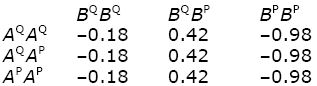
For example, the genotypic value of AQAQ BQBP is –1, which deviates from the mean by –1.82. Since the breeding value is –1.64, the dominance deviation is –1.82 – (–1.64) = –0.18.
|
| iii) |
The additive genetic variance is the variance of breeding values: Va = 0.1764 × (–1.64)2 + 0.1512 × (–0.24)2 + ... + 0.0144 × (3.16)2 = 1.3032. The dominance variance is the variance of dominance deviations: Vd = 0.1764 × (–0.18)2 + 0.1512 × (0.42)2 + ... + 0.0144 × (–0.98)2 = 0.1764. As a check, Va + Vd = 1.3032 + 0.1764 = 1.4796 = Vg.
|
| iv) |
The genotypic values have a roughly square distribution (0.1764, ..., 0.0816; Fig. P14.8, red bars). Allowing for VE = 0.49, each genotype has a normal distribution (Fig. P14.8, thin black lines). Adding these up gives a roughly normal phenotypic distribution (Fig. P14.8, thick black curve). This differs slightly from a normal distribution with the same mean and variance (Fig. P14.8, blue curve), but this difference would be undetectable unless the sample were extremely large.
|
|
Answer 14.6
|
| i) |
The genotypic values, and the genotype frequencies, are as follows:
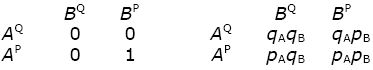
Measuring from the baseline length of AQBQ, and assuming that the alleles are combined at random, or in other words, are in linkage equilibrium).
A fraction 1 – pApB has value 0, and pApB has value 1. The mean is pApB, and the overall variance is the average squared deviation from this mean: Vg = (1 – pApB)(–pApB)2 + pApB(1 – pApB)2, which simplifies to pApB(1 – pApB).
An AQ allele will always be in an insect with value 0, whereas an AP allele finds itself with BP with probability pB; its average trait value is therefore pB. The average excesses of alleles of gene A, which are expressed as deviations from the mean pApB, are therefore (–pApB, pB – pApB) = (–pApB, qApB). Similarly, for gene B the average excesses are (–pApB, pAqB). For gene A, we have a fraction qA that contributes –pApB to the breeding value, and a fraction pA that contributes +qApB. The contribution to the additive genetic variance is therefore qA(–pApB)2 + pA(qApB)2 = pAqApB2. Adding the contribution from B, we have VA = pAqApB2 + pA2pBqB. The difference between Vg and VA is the interaction variance, VI. (This can also be written VAA, because it is entirely due to the interaction between two loci.)
Figure P14.9 shows the total genotypic variance (VG, upper curves) and the additive variance (VA, lower curves) plotted against pA; the shaded area represents the interaction variance, VI = VAA. Beige is pB = 0.2, green is pB = 0.5, and blue is pB = 0.8.
|
| ii) |
Over most of the range of allele frequencies, most variance is additive: The interaction variance makes up a large fraction of total variance only when both pA, pB are rare (blue area, lower left). This is because when pA and pB are common, most of the trait variation can be ascribed to the additive effect of each allele, which will often meet the complementary allele needed to express the trait in the population. When both are rare (blue, lower left), the additive effects of each are small, because a pair APBP is unlikely to form by chance. In general, most trait variation can be ascribed to additive effects, even when there is strong underlying epistasis.
|
|
Answer 14.7
|
| i) |
Figure P14.10 shows the distribution of head shape in F2 males, together with the parent species (D. silvestris, left; D. heteroneura, right), and the F1 (center). The variance of each is assumed to be the same as that in the F1, which was given as 0.000067 (i.e., standard deviation 0.0082).
|
| ii) |
If only one gene were involved, the distribution in the F2 would be as shown in the diagram, with 1:2:1 proportions of the three genotypes, at values (1.136, 1.197, 1.298). The mean is (1.136/4) + (1.197/2) + (1.298/4) = 1.207, and the genotypic variance would be Vg = ((1.136 – 1.207)2/4) + ((1.197 – 1.207)2/2) + ((1.298 – 1.207)2/4) = 0.00338. The actual variance is much smaller. If the environmental variance is assumed to be the same as that in F1, then the actual Vg = 0.00055 – 0.000067 = 0.000483. This is much lower than expected for one locus, implying that many genes are involved: More directly, the F2 distribution barely overlaps with the distribution of parents’ phenotypes, implying that it is unlikely that either parental genotype would be found in the F2. On the other hand, if very many additive genes were involved, each F2 individual would have about the same number of alleles from each parent species, and so genotypic values would be clustered tightly around the middle.
|
| iii) |
The estimated number of genes is Δ2/(8Vg), where Vg is the variance in the F2. Hence, n ~ (1.298 – 1.136)2/(8 × 0.000483) ~ 6.8. The assumption here is that the alleles have equal and additive effects. We know that the F1 is not precisely intermediate, so there is some dominance; moreover, it is unlikely a priori that gene effects would be the same across loci.
|
|
Answer 14.8
|
| i) |
Taking the variance of the F1 as an estimate of the environmental variance in the backcross, we estimate the genetic variance in the backcross as (1.29)2 – (0.51)2 = 1.40 for stigma exsertion, and (0.60)2 – (0.28)2 = 0.28 for log(fruit weight). (Recall that the variance is the square of the standard deviation.) Using the formula Vg = Δ2/(4n), where Δ is the difference in means between the F1 and the backcross parent, L. esculentum, we estimate n = 2.2 for stigma exsertion and 1.6 for log(fruit weight). These estimates are low because there is high variance in the backcross, with the range of values overlapping the parents’ values. The data are consistent with approximately two genes of equal and additive effects on these traits.
|
| ii) |
For stigma exsertion, four associations are statistically significant at the 1% level. However, two of these markers are on chromosome 2 and so could be associated with the same QTL. Therefore, we estimate a minimum number of three QTL. Similarly, for fruit weight, we estimate three QTLs. It could be that a single QTL on chromosome 2 affects both fruit weight and stigma exsertion, in which case, the total number of QTLs detected would be five. NOTE 14F
|
| iii) |
The sum of the 12 estimated δ for stigma exsertion is Σδ = –2.81; these are defined as the difference between E/E and E/P genotypes at each locus. Including just the three chromosomes with significant associations gives a total of –0.88 – 0.90 – 0.74 = –2.52 if we take the QTL on chromosome 2 as having average effect 0.90. The difference between L. esculentum (all E/E) and the F1 (all E/P) is Δ = –1.78 – 1.77 = –3.55. Thus, the total of the estimated QTLs accounts for most, but not all, of the entire difference in means between the parents. Since the estimates have much error, and vary in sign, and since the actual QTLs must have larger effects than these estimates (see below), we can account for the total difference as being the sum of effects of the QTL. For log(fruit weight), Σδ = 1.01 (0.37 if only the three significant QTLs are counted), whereas Δ = 2.31 – 0.95 = 1.36. Again, the estimated QTLs’ account for most of the overall difference, although now we must include all of the nonsignificant estimates.
By adding up the observed δ, we are assuming that linkage is tight, so that the δ equal the effects of the QTLs. If instead there is a recombination rate c = 0.20, the QTLs effect is 1/(1 – 2c) = 1.67 times larger. This now accounts for the overall difference.
|
| iv) |
The QTLs for stigma exsertion presumably vary in the directions of their effects, so that the parents differ by a mixture of alleles with positive and negative effects. This implies that the backcross should include genotypes with values outside the range of the parents, as is seen in the first table (top right). In contrast, QTLs for fruit weight all act in the same direction, and backcross individuals are almost all within the range of their parents. (The range extends down to 0.75, which slightly overlaps the F1 distribution.)
This difference is likely because the cultivated variety has been selected for fruit weight, so that it is fixed for alleles with entirely positive effects. In contrast, there may have been little or no directional selection on stigma exsertion. NOTE 14G
|
|
Answer 14.9
|
| i) |
Marker alleles that are linked to alleles that make Plasmodium drug-sensitive will be eliminated from the population along with the sensitive alleles. Thus, a localized drop in the frequency of sensitive marker alleles from the sensitive strain indicates the presence of a gene that influences drug resistance.
|
| ii) |
Initially, we expect all the alleles that differ between the parent strains to be at 50% frequency; the drug-sensitive allele (dhfrS) is assumed to be eliminated by the time of sampling. Consider a single marker locus, with alleles MR, MS. With a recombination rate c, we start with four genotypes in the following proportions:
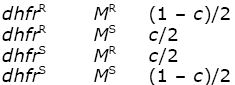
At the end, we just have the resistant allele at the dhfr locus, and so the frequency of the MS allele among the survivors is just c. We predict that the relative intensity will increase in proportion to c. Figure P14.11 shows the observed data, with the best-fitting straight line through them. NOTE 14H
|
|
Answer 14.10
|
| i) |
The homozygote for the high-risk allele (call it FTOP) is at frequency 0.16. Assuming Hardy–Weinberg proportions, p2 = 0.16, and so the frequency of the allele itself is p = 0.40. The genotype frequencies are 0.16:0.48:0.36.
|
| ii) |
The average relative risk is 1.67 × 0.16 + 1.30 × 0.48 + 1 × 0.36 = 1.251. The average rate of obesity overall is given as one in five (0.20), and so the absolute risks for the three genotypes are 0.267:0.208:0.160. Assuming that the environment stays the same, the rate of obesity would increase from 0.2 to 0.267 if FTOP were fixed and decrease to 0.16 if it were eliminated.
|
| iii) |
The FTOP allele cannot have increased quickly enough to have had any appreciable effect on rates of obesity: These are stated to have tripled during the past approximately 20 years, which is less than one generation. In any case, even a complete substitution of one allele for the other would only increase the rate of obesity by a factor 1.67.
Another interpretation of the opening sentence could be that most of the extra cases of obesity are individuals homozygous with this allele. But, the relative risk over the present population averages 1.251, and so only 25% of cases of obesity can be attributed to the presence of the FTOP allele. This opening sentence is a wild exaggeration.
|
References
Bulmer M.G. 1985. The mathematical theory of quantitative genetics. Oxford University Press, Oxford.
Orr H.A. 1998. Testing natural selection vs. genetic drift in phenotypic evolution using quantitative trait locus data. Genetics 149: 2099–2104.
|
|
|

