Evolution Chapter 14 Problems
|
Problem 14.1
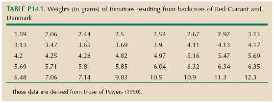
The F1 from a cross between the tomato strains Red Currant and Danmark were backcrossed to Danmark (Fig. 14.3). Table P14.1 shows the weights of 40 tomatoes from this backcross, in grams.
|
| *i) |
To see whether these follow a normal distribution, one can make a histogram and compare it with the normal curve with the same mean and variance (as in Fig. 14.3). A better way is to plot the data as follows. Calculate the mean ( ) and standard deviation ) and standard deviation  and then express the data as deviations from the mean, relative to the standard deviation (i.e., (z – )/ ). Then, plot the data with this deviation on the x-axis, and with each point on successive lines, starting at 0. (In Fig. P14.1, the first few points are plotted in this way.) If these follow a normal distribution, they will lie on the red curve. (This curve shows the probability that a normally distributed variable will be below a given value, measured in standard deviations. For example, the chance of being below –2 standard deviations is approximately 0.025, shown by the first line at 1/40). and then express the data as deviations from the mean, relative to the standard deviation (i.e., (z – )/ ). Then, plot the data with this deviation on the x-axis, and with each point on successive lines, starting at 0. (In Fig. P14.1, the first few points are plotted in this way.) If these follow a normal distribution, they will lie on the red curve. (This curve shows the probability that a normally distributed variable will be below a given value, measured in standard deviations. For example, the chance of being below –2 standard deviations is approximately 0.025, shown by the first line at 1/40).
|
| **ii) |
If fruit weight were normally distributed, what proportion of tomatoes would be predicted to have negative weight?
|
| *iii) |
The F1 has a mean fruit weight of 2.25 g and a variance of fruit weight of 0.71 g2. Estimate the heritability of fruit weight in the backcross population. HINT 14A
|
| **iv) |
Now, take logs of the data and calculate the mean and standard deviation of these transformed data. When plotted in the same way, are they closer to a normal distribution? HINT 14B
|
| **v) |
The F1 has a mean log fruit weight of 0.32 and a variance of log(fruit weight) of 0.026 (using logarithms to base 10). What is the heritability of log(fruit weight) in the backcross population?
|
|
Problem 14.2
Table P14.2 shows how the mortality of two strains of insects (P1, P2) increases with concentration of insecticide; the mortality of the F1 and F2 crosses between these strains is also shown. Each entry gives the number of individuals that died out of a sample of 100.
Assume that individuals have an underlying threshold dose and die if the actual concentration exceeds this threshold (Fig. 14.4). The concentrations shown in Table P14.2 span a very wide range, and so it is natural to use a log scale; assume that the threshold is normally distributed on this scale.
|
| **i) |
What is the mean and variance of this threshold in the parental lines, the F1 and the F2? HINT 14C
|
| **ii) |
What is the heritability of the threshold in the F2 population?
|
|
Problem 14.3
Figure 14.5C shows the heights of father and son, for just over 1000 pairs. The variance of fathers’ height is 7.40 inches2, the variance of sons’ height is 7.54 inches2, and the covariance between the two is 3.84 inches2.
|
| **i) |
Estimate the additive genetic variance of height and its heritability for the population of sons. HINT 14D
|
| **ii) |
Similarly, the variance of mothers’ heights is 5.63 inches2, and the covariance between mothers’ and sons’ heights is 3.23. Estimate the additive genetic variance of height and its heritability, as in i). HINT 14E
|
| **iii) |
Figure P14.2 shows the joint distribution of father’s height and mother’s height. The covariance between these two is 1.84 inches2. What is the correlation between the heights of the parents? What effect will this correlation have on the estimates of heritability in (i) and (ii)? (Just give a qualitative answer.) HINT 14F
|
| ***iv) |
The covariance between brothers’ heights is 3.65 inches2, based on a sample of 328 pairs. What does a comparison between this covariance and the covariance between parent and offspring tell you? HINT 14G
|
|
Problem 14.4
An allele in a diploid plant increases flower size: One copy triples it, and a second copy triples it again. The frequency of this allele is at 20%.
|
| **i) |
What are the genotypic values, the mean flower size, the breeding values, and the dominance deviations? HINT 14H
|
| **ii) |
What are the genotypic variance, the additive genetic variance, and the dominance variance?
|
| **iii) |
Now, suppose that the allele frequency increases to 80%. What are the variance components now?
|
| **iv) |
If we work with log(flower size), what are the variance components?
|
|
Problem 14.5
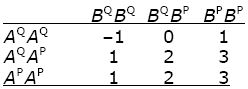
Suppose that two genes, each with two alleles, influence a trait. Following Box 13.1, we call these alleles AQ, AP at gene A, and BQ, BP at gene B; their frequencies are qA = 0.6, pA = 0.4 and qB = 0.7, pB = 0.3. Gene A has additive effects –1, 0, and +1, whereas allele BP is dominant, with effect +2. The effects of the two loci add up. Thus, the phenotypes are as follows.
|
| *i) |
Assuming that the alleles at different genes are combined at random, what are the frequencies of the nine genotypes? What are the frequencies of the five genotypic values (–1, 0, 1, 2, 3)? Calculate the genotypic variance, VG. HINT 14I
|
| **ii) |
What is the average excess of each allele? What are the breeding values and dominance deviations of each genotype?
|
| *iii) |
Calculate the variances of these two quantities; these are the additive genetic variance VA and the dominance variance VD. Do these account for the entire genotypic variance (i.e., VA + VD = VG)?
|
| ***iv) |
Draw a histogram showing the distribution of genotypic values. Assuming an environmental variance VE = 0.49 and assuming that environmental deviations are normally distributed, sketch the distribution of phenotypes. Is this close to a normal distribution? HINT 14J
|
|
Problem 14.6
Antenna length in a haplodiploid insect is influenced by two genes, each with two alleles (AQ, AP and BQ, BP). (Recall that in a haplodiploid, fertilized eggs develop into diploid females and unfertilized eggs develop into haploid males; see p. 666.) These alleles show complete epistasis: In males, APBP have antennae that average 1 mm longer than those of the other three genotypes.
|
| ***i) |
Draw a graph showing the variance components in males as a function of the allele frequencies pA, pB. HINT 14K
|
| **ii) |
How can you explain the changes in relative contributions from the different variance components? HINT 14L
|
|
Problem 14.7
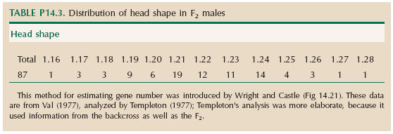
The two species of fly, Drosophila heteroneura and Drosophila silvestris (see Fig. P14.3) are found on Hawaii and are closely related. They differ in head shape, with D. heteroneura having a wide head that is used in courtship display. Head shape was measured from males from populations of each species and for the F1 and F2 of a cross between them. (The measure describes the width of the head relative to its length.) Male D. heteroneura have a mean shape 1.298, whereas D. silvestris have a mean shape 1.136. The F1 have mean 1.197, and variance 0.000067. Table P14.3 gives the distribution of head shape in 87 F2 males; the mean is 1.223 and the variance is 0.000565.
|
| *i) |
Plot the distribution of head shape in the F2; indicate the distributions of parental and F1 populations.
|
| **ii) |
If one gene were responsible for the shape difference, what would be the distribution? What is its variance? If very many genes were responsible, what would the variance be? HINT 14M
|
| **iii) |
Assuming that n genes with equal and additive effects are responsible for the shape difference, the variance in the F2 is predicted to be Δ2/(8n), where Δ is the difference in means between parents. Estimate the number of genes involved, n. HINT 14N
|
|
Problem 14.8
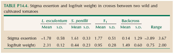
A cross was made between a line of cultivated tomatoes (Lycopersicon esculentum) and its wild relative, Solanum penillii. The F1 was then backcrossed to L. esculentum. Fruit weight and stigma exsertion were measured on each plant. (The stigma is inserted into the flower in the cultivated variety—a trait associated with self-fertilization—but exserted outside the flower in the wild species.) Table P14.4 shows the means and standard deviations and the range of values seen in the backcross. Because fruit weight varies so much between wild and cultivated tomatoes (2.73 g vs. 205.10 g), it is expressed on a log scale (recall Problem 14.1). (We use logs to base 10.)
|
| *i) |
If the differences between the two parental lines are due to n genes of equal effect, all acting in the same direction, then the genetic variance in the backcross is Δ2/(4n); Δ is the difference between the F1 and the backcross parent. (This formula is similar to that in the previous problem, which applied to an F2.) Estimate the number of genes responsible for differences in the two traits.
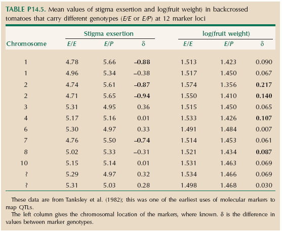
This Wright–Castle estimate is described on page 399 and in Figure 14.21. It is a crude method, which makes the drastic assumption of equal effects and takes no account of genetic linkage. A far more powerful method is to map quantitative trait loci (QTLs) through associations between genetic markers and the traits (p. 399). The backcross plants were scored for 12 allozymes, which are fixed for different alleles in the parental lines (labeled E, P); backcross plants inherit either an E allele or a P allele from the F1 parent, and so have genotype E/E or E/P. Table P14.5 shows the mean trait values of plants with either genotype, for each of the 12 allozyme loci, and also the difference between these means (δ). Differences that are statistically significant at the 1% level are marked in bold. The chromosome on which each marker is located is shown. These species have 12 chromosomes; two marker locations are unknown.
Differences in trait mean, δ, between genotypes indicate linkage to a QTL (Box 14.3). If the QTL is tightly linked, then δ estimates the size of its effect, α. However, if it is loosely linked, then it must have a larger effect, which is only partially reflected in δ. With recombination rate c between the marker and the QTL, δ = α(1 – 2c).
|
| **ii) |
What is the minimum number of QTLs that influence the two traits? HINT 14O
|
| **iii) |
Does the total effect of all the QTLs that are detected in the backcross account for the differences (Δ) between the F1 and L. esculentum? Assume either that the detected QTLs are completely linked (c = 0) or that on average, c = 0.20. HINT 14P
|
| ***iv) |
Why do some marker effects on stigma exsertion, δ, go in the direction opposite to the difference beween the parents? Why might fruit weight show a more consistent pattern than stigma exsertion?
|
|
Problem 14.9
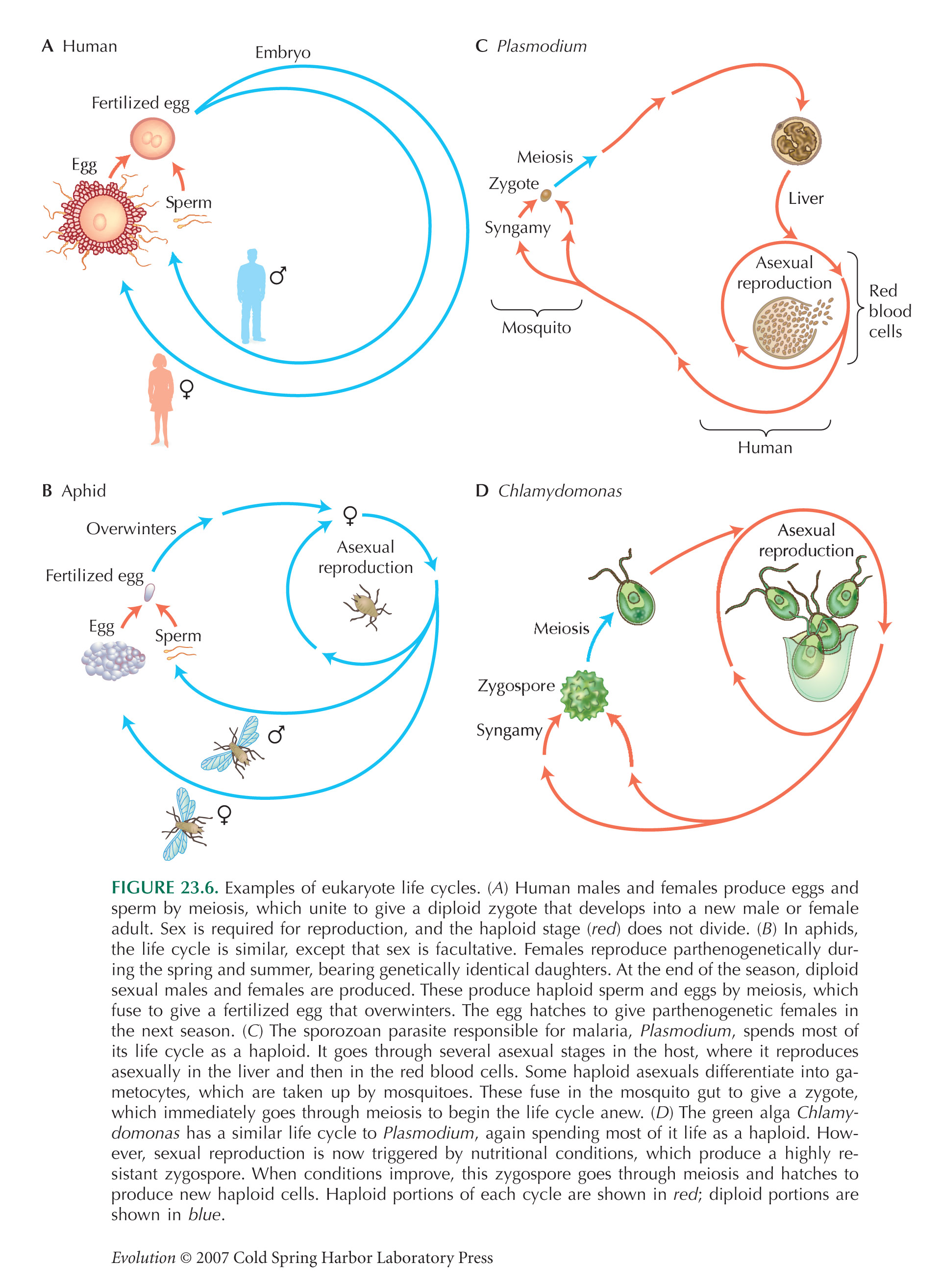
This problem is based on a method for mapping genes for drug resistance in the malaria parasite. The parasite that causes rodent malaria, Plasmodium chabaudi, is haploid for most of its life cycle. It reproduces asexually within the rodent host and is taken up by mosquitoes when they take a blood meal. Haploid gametocytes within the mosquito unite to form a diploid zygote, which immediately goes through meiosis to produce haploid offspring that can be transmitted to a new rodent host (see Fig. 23.6C).
A cross was made between two strains of P. chabaudi, one of which was resistant to the drug pyrimethamine. This was done by allowing mosquitoes to feed on mice that had been infected with both strains in equal proportions. Thus, these mosquitoes produced a mixture of offspring from crosses within and between strains. These offspring were grown up in mice that had been treated with pyrimethamine. They were then sampled, and their DNA was pooled. Finally, these pooled samples were scored for the frequency of markers that differed between the parent strains. (The intensity of binding to a marker sequence from the sensitive strain is proportional to its frequency in the population of offspring.)
Figure P14.4 shows the relative intensity of binding to marker sequences along the genome. Each stripe shows markers on one chromosome.
Table P14.6 shows the relative intensity of binding for six markers, together with their map distance from a candidate gene for drug resistance, dhfr. (Map distance is measured in centiMorgans; the recombination rate c is found by dividing by 100.)
|
| **i) |
Explain why the marker intensity varies between these markers. HINT 14Q
|
| **ii) |
What marker intensity would you predict if the dhfr allele from the sensitive strain has been eliminated from the population of Plasmodium that grew up in pyrimethamine-treated mice? Draw a graph that compares the observed marker intensity with this prediction. HINT 14R
|
|
Problem 14.10
This is an extract from an article in the Guardian (April 13, 2007; http://www.guardian.co.uk/uklatest/story/0,,6554193,00.html).
Gene could be to blame for obesity
A common gene variant found [homozygous] in 16% of the population could be largely responsible for exploding rates of obesity, it has been revealed.
People with two copies of the gene are almost 70% more at risk of being obese than those having none, and three kilograms heavier on average.
Obesity rates in England have more than tripled since the 1980s. Around one in five adults are obese and more than half either obese or overweight—almost 24 million people.
The obesity gene was identified by a population-wide screening study led by scientists from the Peninsula Medical School in Exeter and the University of Oxford. DNA samples from more than 38,500 people from across the UK and Finland showed a strong association between a particular variation of a gene called FTO and obesity.
Genes come in pairs, and individuals carrying one copy of the FTO mutation were found to have a 30% higher risk of being obese than those with no copies. The increased risk rose to 67% for people who had two copies of the gene variant. ...”
|
| *i) |
What are the frequencies of the three genotypes at the “obesity gene”?
|
| *ii) |
The relative risk of being obese for the three genotypes is given as 1:1.30:1.67. What is the average relative risk in the population as a whole? What would the rate of obesity be if the high-risk allele were lost from the population? If it were fixed?
|
| **iii) |
What might be meant by the first sentence of the article?
(The article was based on a paper by Frayling et al. [Science Express, 2007, doi 10.1126/science.1141634].)
|
References
Culleton R., Martinelli A., Hunt P., and Carter R. 2005. Linkage group selection: Rapid gene discovery in malaria parasites. Gen. Res. 15: 92–97.
Pearson K. and Lee A. 1903. On the laws of inheritance in man. I. Inheritance of physical characters. Biometrika 2: 357–462.
Powers L. 1950. Determining scales and the use of transformations in studies of weight per locule of tomato fruit. Biometrics 6: 145–163.
Tanksley S.D., Medina-Filho H., and Rick C.M. 1982. Use of naturally occurring enzyme variation to detect and map genes controlling quantitative traits in an interspecific backcross of tomato. Heredity 49: 11–26.
Templeton A.R. 1977. Analysis of head shape differences between two interfertile species of Hawaiian Drosophila. Evolution 31: 630–642.
Val F.C. 1977. Genetic analysis of the morphological differences between two interfertile species of Hawaiian Drosophila. Evolution 31: 611–629.
Weber K.E., Eisman R., Morey L., Patty A., Sparks J., Tausek M., and Zeng Z.B. 1999. An analysis of polygenes affecting wing shape on chromosome 3 in Drosophila melanogaster. Genetics 153: 773–786.
|

