 |
|
|
|
|
Evolution Chapter 17 Answers
|
Answer 17.1
|
| i) |
The ratio (p/q) is initially very close to p0 = 10–5 and changes each generation by a factor 1.1. After ten generations, therefore, (p10/q10) = 1.110 × 10–5 = 2.59 × 10⁻⁵; after 100 generations, it is 1.1100 × 10–5 = 0.138. The two types will be equally frequent when 1.1t = 105, so that t = log(105)/log(1.1) ~ 121 generations.
|
| ii) |
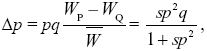
We have
and so
and so
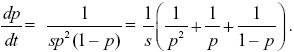
Approximating the change across one generation as the rate of change in continuous time (Δp = dp/dt) and dropping the relatively small term 0.1pt in the denominator, we have

This has the solution
(Chapter 28).
|
| iii) |
Figure P17.3 shows the accuracy of this approximation; allele frequency is shown on a log scale.
The continuous time approximation overestimates the rate of increase. In this simplest case, the continuous and discrete time formulae match exactly if we set the continuous time selection coefficient to loge(1.1) = 0.0953. In general, though, there will be a discrepancy however we choose the parameters. However, this error is negligibly small if selection is weak (s < 0.1, say).
|
|
Answer 17.2
|
| i) |
The rate of increase of an allele with selective advantage s is spq, which is approximately sp for p << 1. The rate of increase due to mutation is μq (because the fraction q of the population can mutate at a rate μ to give the new allele), and this is approximately μ for p << 1. Because both terms are small, we can add them to give dp/dt = sp + μ.
|
| ii) |
Substituting for p = (μ/s)(est – 1) shows that this is a solution. Differentiating est with respect to time gives s est, and so (dp/dt) = μest, which equals sp + μ as required.
|
| iii) |
We have two approximations: p = (μ/s)(est – 1) applies when p << 1 (less than 0.1, say), and p = (μ/s)est/(1 + (μ/s)est) applies when p >> μ/s (which is typically very small). These match each other at (μ/s)est in the intermediate range where both approximations apply: (μ/s) << p << 1. To answer the question, we ned to find when p = 1/2. This is when (μ/s)est = 1 or t = (1/s)loge(s/μ).
|
| iv) |
The strongly selected allele will reach 50% at t = 10 loge(109) ~ 207 generations, whereas the weakly selected alleles will reach 50% at t = 100 loge(1010) ~ 2300 generations. The selection coefficient has a far greater influence than the initial frequency or the mutation rate. See Figure P17.4.
|
|
Answer 17.3
|
| i) |
At equilibrium, WQ = 1 and so N = 1. This is shown in Figure P17.5 as the point where the red curve (WQ) crosses the green line (W = 1).
|
| ii) |
See Figure P17.5.
|
| iii) |
At the initial equilibrium with Q fixed, N = 1 (red line in Fig. P17.5). At that population size, WP = 3/2 and so P will invade; the blue curve lies above the red line at N = 1. As it invades, it displaces Q, and ultimately, the population fixes for P at a higher density (N = 2, WP = 1, WQ = 4/9; arrows in Fig. P17.5).
|
| iv) |
Initially, both Q and P increase, but Q increases faster than P. Once Q reaches its carrying capacity, P continues to increase, and eventually outcompetes Q (Fig. P17.6). Over most of this plot (whenever N > 1/3), P is fitter than Q.
|
|
Answer 17.4
|
| i) |
Write the numbers of juveniles and adults at time t as nJ,t, nA,t. Then
nJ,t + 1 = 0.4nJ,t + 2nA,t ,
nA,t + 1 = 0.4nJ,t .
Over the first ten generations, this gives
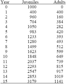
The numbers fluctuate between juvenile and adult, but these fluctuations dampen out. The ratio between numbers in successive generations settles to about 1.12, and the ratio of juveniles to adults settles to about 2.79. This is the general behavior of this kind of recursion: The numbers in the different classes settle to a constant ratio and increase together at a steady rate (see Chapter 28).
We can find this steady rate (known as the leading eigenvalue) using the same method as that in Box 28.3. We look for a solution with
nJ,t + 1 = λnJ,t = 0.4nJ,t + 2nA,t ,
nA,t + 1 = λnA,t = 0.4nJ,t .
The absolute magnitudes of nJ, nA are arbitrary, so we can set nA = 1. This gives a quadratic equation that has two solutions. The solution with the largest magnitude of growth rate is λ = 1.117, nJ = 2.79, as we found above.
|
| ii) |
Using either of the two methods above, we find that the new type has growth rate λ* = 1.2. Relative to the growth rate of the original type, this is λ*/λ = 1.075, corresponding to a selection coefficient of 7.5%. The 20% increase in one fitness component (adult reproductive success) causes a smaller increase in overall fitness, as measured by this steady rate of increase. NOTE 17E
|
|
Answer 17.5
|
| i) |
In the first generation, the fitnesses are {2,2,0,1,2,0,2,2,0,1}; mean fitness is 1.2 and the variance in fitness is 0.844. NOTE 17F
|
| ii) |
The mean fitnesses of the red and blue allele are 2, 0.667, respectively. Subtracting the overall mean, we find that the average excesses are +0.8, – 0.533. The additive genetic variance is the variance of these average excesses: varA(W) = 0.4(0.8)2 + 0.6(–0.533)2 = 0.427.
|
| iii) |
The frequencies of the red and blue alleles among the offspring are 0.667 and 0.333, respectively. Therefore, based on the average fitnesses of these alleles, we predict that the offspring will have mean fitness 0.667 × 2 + 0.333 × 0.667 = 1.556, a change of Δ = 0.356. This is equal to varA(W)/, as predicted by the Fundamental Theorem. = 0.356. This is equal to varA(W)/, as predicted by the Fundamental Theorem.
|
| iv) |
The fitnesses in the next generation are {3,1,2,0,1,1,0,3,0,3,1,1} with mean 1.333. Thus, mean fitness has increased by only 0.133, not 0.356 as predicted. This is because the average fitnesses of the two alleles have changed: The fitnesses of the red and blue alleles were 2, 0.667 in the first generation, but 1.5, 1 in the second. The differences might be due to chance fluctuations in the fitnesses of the small numbers of each allele, or they might be due to a change in environment. Fisher’s Fundamental Theorem only predicts the change in mean fitness due to natural selection on allele frequencies, holding the effects of each allele constant.
|
|
Answer 17.6
|
| i) |
Figure P17.7 shows which genes were transmitted to each offspring. Because one cannot know which parent transmitted which gene simply from the genotypes of diploid parents and offspring, this is one of several valid solutions.
|
| ii) |
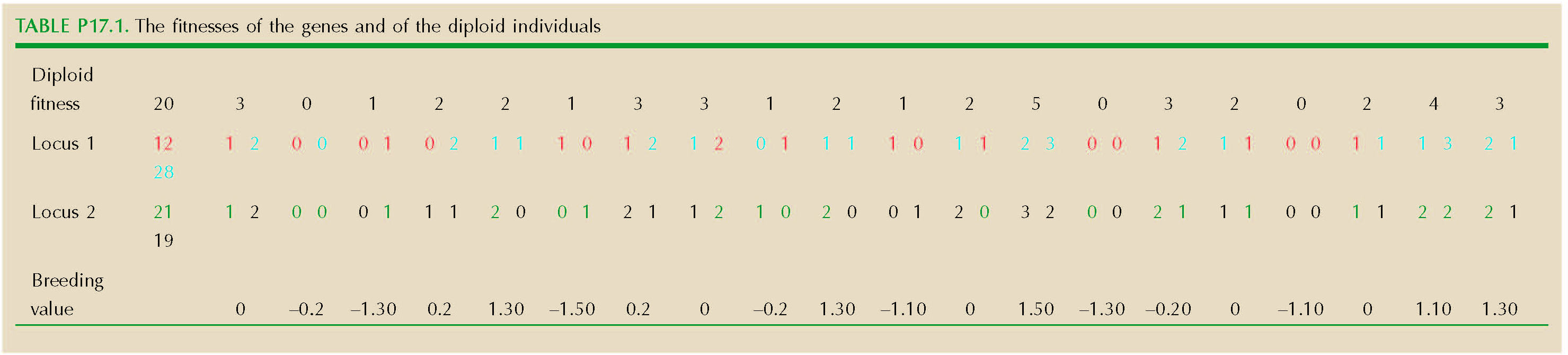
See Table P17.1. The total variance in fitness at the first locus is 0.65 and at the second, 0.7.
The average excess of an allele is defined as the average fitness of genes carrying that allele minus the overall average. This is –0.4, +0.4 for the red and blue alleles at the first locus and 0.05, –0.05 for green and black alleles at the second locus. The additive genetic variance in fitness is just the variance of the average excess. Alleles are at 50% frequency at both loci, and so varA(W) = (1/2)(–0.4)2 + (1/2)(0.4)2 = 0.16 for the first locus and, similarly, 0.0025 for the second locus. Only a fraction of the genetic variance fitness can be attributed to the effects of these alleles.
At the first locus, there are 28 copies of the blue allele and 12 copies of the green among the offspring. We estimated that the blue allele increases mean fitness by 0.4 and the red reduces it by 0.4, and so the increase in mean fitness due to the increased frequency of the blue allele is –0.4(12/40) + 0.4(28/40) = 0.16. The mean fitness is 1, and so Fisher’s Fundamental Theorem is precisely true: Δ = varA(W)/; the same is true for the second locus.
|
| iii) |
Usually, we work with diploid individuals, not the individual genes that they carry. Their fitnesses are given in Table P17.1; the total variance of individual fitness is 1.700. The fitnesses of the three genotypes at each locus are
Therefore, the mean fitnesses of the red, blue alleles are 1.35, 2.65 and of the green, black alleles 1.9, 2.1, respectively. The average excesses are therefore –0.65, +0.65 at the first locus and +0.1, –0.1 at the second. By adding these average excesses over the four genes in each individual (two at each locus), we get the breeding value (Table P17.1, bottom row). The variance of breeding value gives the additive variance as varA(W) = 0.839. NOTE 17G
Allele frequencies change from 0.5 at both loci to 0.3, 0.7 for the red, blue alleles and 0.525, 0.475 for the green, blue alleles. Therefore, the change in mean fitness due to changed allele frequencies is 2(–0.65 × 0.3 + 0.65 × 0.7) + 2(+0.1 × 0.525 – 0.1 × 0.475) = 0.530.
This is rather more than the prediction from the Fundamental Theorem, varA(W)/ = 0.839/2 = 0.420. This is primarily because the fitness of a diploid individual does not exactly predict the fitnesses of the genes that it carries—this depends on which genes are transmitted at meiosis. Thus, a gene that was preferentially transmitted would increase in frequency even if there were no variance in the fitness of individual diploids. (We examine the consequences of such non-Mendelian transmission in Chapter 21.) In this example, the slight discrepancy may just be due to random segregation in the small number of individuals. NOTE 17H
To sum up, Fisher’s formula gives an exact prediction of just one component of the change in mean fitness: that caused by natural selection on allele frequencies. It does not include the effects of changes in environment, of nonrandom associations between genes, or (when applied to diploids) of uneven transmission at meiosis.
|
|
Answer 17.7
|
| i) |
When P is rare, PP homozygotes hardly ever form, and so the relative fitnesses of the P and Q alleles are determined by the relative fitnesses of the PQ and QQ genotypes. Over a cycle of ten generations, the frequency of allele P will change by a factor 2 × 0.99 = 0.775. This corresponds to a ratio of 0.7751/10 = 0.975 per generation. (This is the geometric mean fitness; see p. 469.) The P allele cannot invade: It will decrease by (on average) 2.5% per generation when introduced at low frequency.
|
| ii) |
Now, the A patches contribute 90% of the whole population, and the proportion of PQ heterozygotes within patches declines by a factor 0.9; B patches contribute 10% of the population and the proportion of PQ heterozygotes within them increases twofold. The net proportion therefore changes by 0.9 × 0.9 + 0.1 × 2 = 1.01. (This is the arithmetic mean.) The P allele increases by 1% per generation.
|
| iii) |
Now, we do the same analysis, but using the ratio between the fitnesses of the rare PQ heterozygote and the predominant PP homozygote. With temporal variation (i), Q increases from low frequency by a factor (0.9/0.8)9 + (2/2.1) = 2.75 over ten generations, or 2.751/10 = 1.11 per generation. Thus, P cannot invade Q and Q can invade P: Q will always fix, regardless of the starting frequencies. With spatial variation (ii), Q increases from low frequency by a factor 0.9(0.9/0.8) + 0.1(2/2.1) = 1.11, and so Q can invade P. Because P can also invade Q, there must be a polymorphism. NOTE 17I The average fitnesses of QQ:PQ:PP are 1:1.01:0.84 (taking the arithmetic mean over patches) and so this polymorphism is maintained by net heterozygote advantage.
|
|
Answer 17.8
|
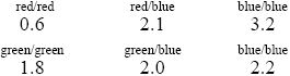
| i) |
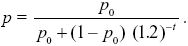
At equilibrium, the two patterns must give equal fitness. Therefore, 0.6 = 1 – 0.9u, and so the frequency of the pattern is u = 4/9. Assuming Hardy–Weinberg proportions, u = p2 and so p = 2/3.
|
| ii) |
When the pattern is rare, the relative fitnesses of the two phenotypes are 0.6:1. However, the conspicuous pattern is determined by a recessive allele, and so the two alleles have almost the same fitness: The fitter PP homozygote is rarely formed. The Q allele is always in the cryptic pattern and has fitness WQ = 0.75, whereas the P allele finds itself in a butterfly with the conspicuous pattern with probability p, and so has fitness WP = 0.6(1 – p) + p. The P allele therefore increases from p to p(WP/WQ) = p(1 + 2p/3); the change in allele frequency is Δp = 2p2/3. If the pattern is at 0.01, then the corresponding allele is at p = 0.1 and Δp = 0.00667. The change in frequency of the conspicuous pattern is (0.10667)2 – 0.01 = 0.00138. Increase of a favorable recessive allele from low frequency is very slow.
When the conspicuous pattern is at high frequency, the patterns have relative fitnesses 0.6:0.1. Since the population consists almost entirely of PQ, PP genotypes, the Q allele increases from q to q(0.6/0.1) = 6q. The dominant Q allele invades very rapidly.
We can also get the answer using the formula in Box 28.1. We have
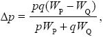
where WQ = 0.6, WP = 0.6q + (1 – 0.9p2)p. Hence,
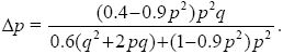
When p << 1, q ~ 1 and Δp ~ 0.4p2/0.6; when q << 1, p ~ 1, and Δp ~ – 0.5q/0.1, which is consistent with the calculations above.
|
| iii) |
At equilibrium (p = 2/3), the phenotypes have frequencies 5/9, 4/9 and both necessarily have the same fitness, 0.6. However, at p = 1/2, the phenotypes have frequencies 3/4, 1/4 and fitnesses 0.6, 1 – 0.9(1/4) = 0.6, 0.775 and so mean fitness is 0.644, higher than at equilibrium (see Fig. P17.8). Actually, we can immediately see that at equilibrium, both phenotypes must have fitnesses 0.6, which is the same as if they were all cryptic. NOTE 17J
|
|
Answer 17.9
|
| i) |
Assuming random mating, so that the P allele finds itself in a PP homozygote with probability p, the fitnesses of the two alleles are WQ = 1, WP = 1 + sp; the mean fitness is = 1 + sp2. From Box 28.1,
where q = 1 – p.
|
| ii) |
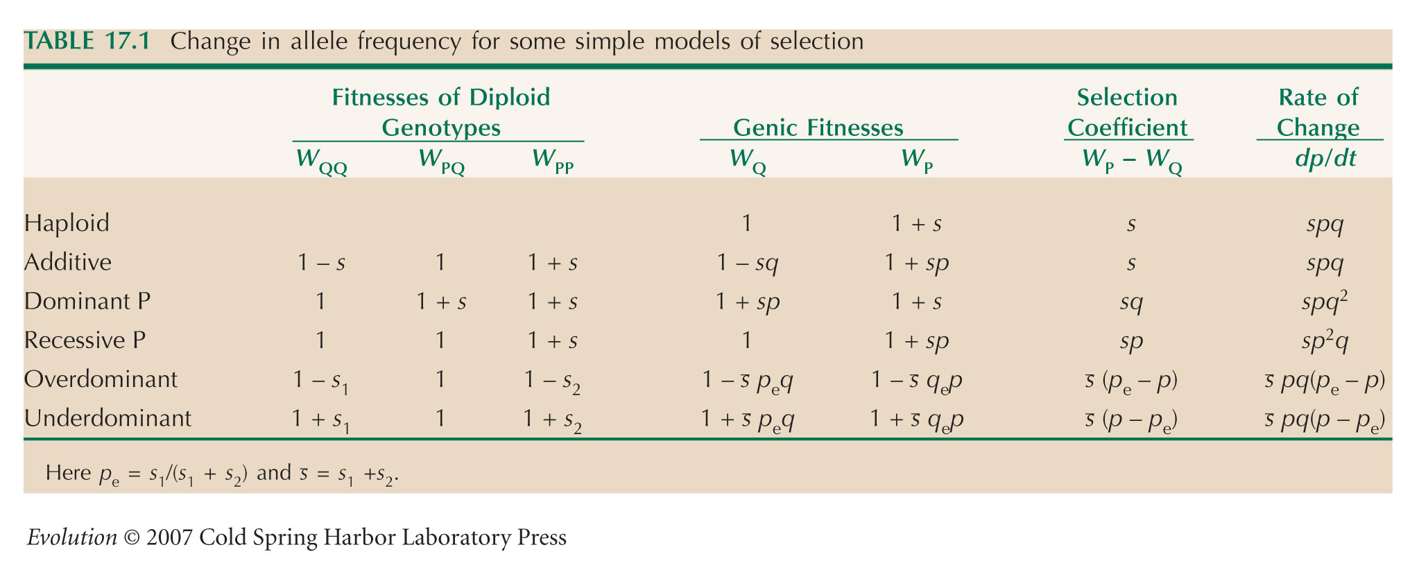
When selection is weak (s << 1), this is closely approximated by

(as given in Table 17.1).
|
| iii) |
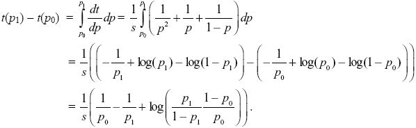
Following the same method as that in Box 28.2, we can integrate this equation to find the time taken for the allele frequency to change from p0 to p1:
Thinking of time as a function of allele frequency, t(p) NOTE 17K;
|
| iv) |
Substituting into the formula above, we find that it takes about 10,820 generations for the recessive allele to increase from 0.01 to 0.99 and about 106 generations to increase from 0.0001. This last figure is close to 1/(sp0), which is the dominant term in the formula for small p0.
|
| v) |
We can find the corresponding times for an additive allele by substituting into the formula in Box 28.2, with s = 0.005. (This ensures that the difference in fitness between PP and QQ is the same in both cases.) Then, it takes 460 generations to increase from 0.01 to 0.99 and 690 generations to increase from 0.0001 to 0.99. To a good approximation, if the total difference in relative fitness between homozygotes is s, a recessive allele will take ~1/(sp0) to increase, whereas an additive allele takes ~ (2/s)log(1/p0) generations, which is much less time for small p0.
|
| vi) |
If the heterozygote has a slight advantage of 0.001, the fitness of the Q allele becomes 1 + 0.001p, and of the P allele, 1 + 0.001q + 0.01p. Therefore, if p is smaller than ~0.1, the P allele gains greater fitness from its effect on the heterozygote than from its effect on the much rarer homozygotes. To a good approximation, the time taken to increase from 10–6 to high frequency will be the same as that for an additive allele (Box 28.2); we can ignore the effect on the homozygote, because that only contributes right at the end of the process. Substituting into the formula in Box 28.2, with s = 0.001, we calculate a time ~13,800 generations to increase from 0.0001 to 0.99. A slight effect on the heterozygote is much more important than a stronger effect on the homozygote when the allele is rare. In practice, therefore, rare alleles can never be treated as strictly recessive. NOTE 17L
|
|
Answer 17.10
|
| i) |
Assuming that the genotype frequencies are given by multiplying the allele frequencies, the mean fitness is = qAqB × 1 + qApB(1 + s) + pAqB(1 + s) + pApB × 0 = 1 + s(qApB + pAqB) – pApB (where qA = 1 – pA , etc.; here we have used qAqB + qApB + pAqB + pApB = 1). NOTE 17M See Figure P17.9.
|
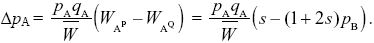
| ii) |
AQ has average fitness WAQ = qB + (1 + s)pB = 1 + spA, whereas AP has average fitness WAP = (1 + s)qB. So, from Box 28.1,
|
| iii) |
Differentiating the expression for in i) with respect to pA, we find that NOTE 17N
|
|
Answer 17.11
|
| i) |
There are two copies of each gene in a diploid, and so an increase in allele frequency Δp of an allele with effect α increases the mean by R = 2αΔp.
|
| ii) |
From the definition of the selection gradient, W = (1 + β(z –  )). The allele increases the trait value by α and so increases fitness by βα. Therefore, from Box 28.1, allele frequency increases by Δp = pq(WP – WQ)/ = αβpq. The change in the trait mean is thus R = 2αΔp = 2α2pqβ. )). The allele increases the trait value by α and so increases fitness by βα. Therefore, from Box 28.1, allele frequency increases by Δp = pq(WP – WQ)/ = αβpq. The change in the trait mean is thus R = 2αΔp = 2α2pqβ.
|
| iii) |
Each gene copy has probability p of increasing the trait by α. So, the mean effect is αp, and the variance in effect (which is defined as the average squared deviation from the mean) is p(α – αp)2 + q(–αp)2 = α2pq. The additive variance contributed by the two copies of this gene in a diploid is therefore 2α2pq. We see that R = VAβ, as required.
|
|
Answer 17.12
|
| i) |
In each generation, additive variance is reduced by VA/2Ne as a result of random drift (see p. 418). Balancing this against the increase VM due to mutation, we have VA = 2NeVM = VE. Therefore, we expect a heritability of h2 = 50%. (See also Problem 15.4.)
|
| ii) |
The rate of change of the mean is R = h2S = 0.5 × 0.4  = 0.2 per generation. = 0.2 per generation.
|
| iii) |
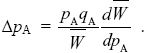
S = βVP, and so the selection gradient is β = S/VP = 0.4 /VP = 0.2/. Thus, an allele that increases the trait by one environmental standard deviation, , increases relative fitness by s = αβ = 0.2; the fitness of the allele is increased from WP = 1 to WP = 1.2. NOTE 17O
|
| iv) |
The increase in trait mean due to this allele is 2αp; the factor of 2 arises because each diploid individual has two copies of the gene. The substitution of the allele is equivalent to ten generations of response to selection on the variation produced by the background of mutations of small effect. The genetic variance it contributes is 2α2pq, which has a maximum value of 0.5VE when p = q = 1/2. This is half the genetic variance produced by all the other loci—substantial, but still hard to detect in real data.
The ratio of allele frequencies with WP/WQ = 1.2 is given by Equation 17.2. Rearranging, we find that the allele frequency is
The trait mean increases at a rate of 0.2 per generation because of the original genetic variation and, in addition, increases because of the new allele. Each copy of the allele has effect α = , and so the net increase is 2αp (the factor of 2 arising because there are two copies in each diploid individual). So, the trait mean is (0.2t + 2p), and the genetic variance in the trait is therefore (1 + 2α2pq)VE. See Figure P17.10.
|
| v) |
Each copy of the allele increases fitness by 0.2, because of selection on the trait. However, two copies are lethal. So, the genotype fitnesses are WQQ = 1, WPQ = 1.2, WPP = 0. The fitness of allele Q is WQ = q + 1.2 × p = 1 + 0.2p, whereas the fitness of allele P is WP = 1.2q + 0 × p = 1.2q. These are equal at equilibrium, and so the equilibrium allele frequency must be given by 1 + 0.2p = 1.2q, or p = 0.143. It will then contribute to 2α2pq = 0.24VE—about one-quarter of the variance due to all other mutations. A fraction p2 ~ 0.02 will die each generation because they are homozygous for the recessive lethal.
|
|
|
|

