 |
|
|
|
|
Evolution Chapter 20 Answers
|
Answer 20.1
|
| i) |
The optimal combination is where the contours of average survival just touch the shaded area, which depicts the possible combinations of survival values. Figure P20.4A shows the optimal solutions (blue circles) where eggs are laid equally on A, B (A: vA = vB = 1/ ; mean survival 1/ = 0.707) and where they are laid in proportions 7:24 (B: vA = 7/25, vB = 24/25, mean survival 25/31 = 0.806). ; mean survival 1/ = 0.707) and where they are laid in proportions 7:24 (B: vA = 7/25, vB = 24/25, mean survival 25/31 = 0.806).
|
| ii) |
Now, the optimal place to lay eggs is where they will survive best: They should all be laid in B (i.e., α = 1).
|
| iii) |
The best place to lay eggs is in whichever host gives higher survival. So, complete specialization will be an optimal solution: Either α = 1, vA = 0, vB = 1 or α = 0, vA = 1, vB = 0. A generalist strategy (vA = vB = 1/, α = 1/2) has mean survival 1/, which is lower.
|
| iv) |
Now, suppose that all the individuals have vA = vB = 1/, and a fraction 1 – α = α = 1/2 of eggs are laid on each patch. The numbers surviving on the two patches are (1 – α)vB and αvB, in this case both equal to 1/2 . An individual with survival vA*, vB* will have a chance (1 – α)vA* of landing in patch A and surviving there and will make up a proportion (1 – α)vA*/(1 – α)vA of the population that emerges. So, the overall chance of survival of this type is proportional to
The ESS is when we find a pair of viabilities {vA, vB} such that no other pair can invade. It is easy to see that because the trade-off curve in Figure P20.4 curves outward, any choice of {vA, vB} cannot do better than the ESS of vA = vB = 1/.
|
| v) |
We have seen that if α = 1/2, then the ESS for survival is vA = vB. Clearly, if α = 1, so that all eggs are laid on B, the ESS for survival is to specialize as vB = 1. Similarly, if α is intermediate, the ESS will be to tend to have higher viability on the host that is more commonly encountered. So, if we allow α to evolve, then specialists will evolve, with α = 0 and vA = 1 or α = 1 and vB = 1. If all the individuals in a population specialized on the same patch, the other patch will not be exploited, and there will be a large advantage to individuals that specialize on that patch. Thus, the ESS is for equal proportions of the two specialist types. Then, there will be perfect survival on both patches, and no alternative can do better.
This ESS could be achieved by a genetic polymorphism (see Fig. 18.22) or by a mixed strategy: Individuals might have an equal chance of laying eggs on either host, but if they are on A, they grow up with the appropriate specialist phenotype. NOTE 20F NOTE 20G
|
|
Answer 20.2
|
| i) |
If the expected number of offspring in each year is R, then the expected number produced in year 1 is (1/2)R, in the next, 1/4R, and so on. The total number over a lifetime is thus (1/2)R + (1/4)R + ··· = R. In a sexually reproducing population with equal sex ratio, each mother must produce two offspring to maintain stable population size, and so R = 2.
|
| ii) |
Now, the expected reproductive success is increased from R to 1.01R in year 1. The chance of surviving to year 1 is 1/2 and so the increase in net relative fitness is s = 0.005. The selection coefficient on an allele that increases fecundity in year by 1% is 1% × 2–t, because there is a change 2–t of surviving until generation t.
|
| iii) |
Increasing survival in year 1 by 1% increases the expected number of offspring in every successive year. Therefore, the selection coefficient is just 1% for an increase in the first year, and declines by 1/2 in every successive year. In general, selection pressures decline in later life: This is the fundamental cause of senescence (p. 562).
|
|
Answer 20.3
|
| i) |
The average number of offspring is 0.5 × 3 + 0.5 × 0.2 × 5 = 2; this keeps the population stable. An allele that reduces fecundity by a factor (1 – x) in year 1 reduces fitness by s = x/2, since there is a 50% chance of surviving to reproduce then. If selection acts mainly to eliminate the deleterious allele in heterozygotes (true unless the alleles are completely recessive), then their equilibrium frequency is μ/s = 2μ/x. The proportion of heterozygotes is about 2μ/s, and so the average reduction in fecundity is x × 2 × 2μ/x = 4μ, or a factor 1 – 4μ. Multiplying effects over all loci, we find that the net reduction in fecundity is (1 – 4μ1)(1 – 4μ2)… ~ exp(–2U) = 0.135. (Recall that the mutation rate per diploid genome is U = 2Σiμi.) Each mutation reduces overall relative fitness by x/2, and so by the same argument, the reduction in mean fitness is by a factor exp(–U).
This result can be reached more directly using the fact that when deleterious mutations are eliminated as heterozygotes, and fitnesses multiply across loci, the mean fitness is reduced by exp(–U), regardless of exactly how selection eliminates the mutations (see p. 552).
|
| ii) |
A reduction in fecundity by x in year 2 reduces relative fitness by s = 0.5 × 0.2x = 0.1x, because the chance of surviving to age 2 is 0.1. Because the net reduction in relative fitness must be by exp(–U), regardless of x, and because the ratio between the effect on relative fitness (s) and on fecundity (x) is 0.1, we can see that the reduction in fecundity is by exp(–U/0.1) = 4.5 × 10⁻⁵. Mutation load catastrophically reduces the contribution of older individuals to fitness.
|
| iii) |
What will the effect of deleterious mutations that affect each year class equally be? Suppose that fecundity is reduced by a factor (1 – x) in both years. Then, relative fitness is just reduced by s = x. By the same argument as above, fecundity is reduced by a factor exp(–U).
|
|
Answer 20.4
|
| i) |
The chance of surviving to the first year is J, and to the second year, J × A. Because fecundity is the same in each year, overall fitness is proportional to J + J × A. We can find the maximum fitness, given the constraint that J + A4 ≤ 1, by plotting contours of fitness against the trade-off curve (Fig. P20.6). The contours are relatively flat, reflecting the greater weight given to juvenile survival (vertical axis) compared with adult. Thus, the optimal life history is J = 0.945, A = 0.484. The increase in mortality with age implies senescence.
|
| ii) |
A 1% decrease in J will decrease fitness by 1%, and so s = 0.01. Total fitness is J(1 + A), and so this is a decrease in A by δA = 1% will decrease fitness by JδA. This is a decrease in relative fitness by δA/(1 + A), or s = 0.0067. Selection is weaker in later life.
|
|
Answer 20.5
|
| i) |
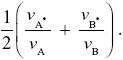
Half of the T alleles will be transmitted through females. Because all females have the same number of offspring, this transmission is random, and a fraction p carries allele TP. Of the other half, a fraction (1 – u) is transmitted via matings with PV females, who have no preference, and so again, the frequency of TP alleles in this class is just p. Finally, those transmitted through males, via matings with PU females, must be type TP, because there is an absolute preference. Therefore,
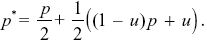
With some rearrangement, we find that
|
| ii) |
After one generation, starting from very low frequency (p << 1, q ~ 1), TP will immediately increase to frequency u/2, because the fraction u of PU females will all mate with TP males. The factor of 2 arises because the males’ allele has a chance 1/2 of being passed on at meiosis. NOTE 20H
|
| iii) |
We know that the preference allele is not directly selected. Therefore, the frequency of the PV, PU alleles that are associated with TP does not change as a result of nonrandom mating. The overall frequency of PU changes from u = puP + quQ to u* = p*uP + q*uQ, and the change in frequency is just Δu = u* – u = Δp(uP – uQ). NOTE 20I This is the change in allele frequency before meiosis. However, recombination does not alter overall allele frequency (see p. 669), and so this formula applies from one generation to the next.
|
| iv) |
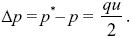
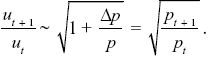
Given that uP – uQ = u/2p, Δu = Δp(uP – uQ) = (u/2p) Δp. This gives the change in allele frequency Δu = ut+1 – ut. So, the ratios change as
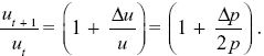
Using the approximation that (1 – x/2) ~  , we find that , we find that
|
| v) |
To find the overall change, we just multiply together the ratios over successive generations:
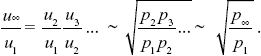
Because the preferred allele eventually fixes, p∞ = 1. We saw in ii) that p1 = u1/2, and so we have u∞ ~  . For example, if the preference allele PU is initially at u1 = 0.01, it will cause the substitution of the preferred allele TP. Because PU favors matings with TP, it will become associated with it. Therefore, as TP fixes, it will take PU with it, increasing it to . For example, if the preference allele PU is initially at u1 = 0.01, it will cause the substitution of the preferred allele TP. Because PU favors matings with TP, it will become associated with it. Therefore, as TP fixes, it will take PU with it, increasing it to  = 0.14. (An exact calculation shows that u∞ = 0.153 for these parameters.) NOTE 20J (See Fig. P20.7.) = 0.14. (An exact calculation shows that u∞ = 0.153 for these parameters.) NOTE 20J (See Fig. P20.7.)
|
|
Answer 20.6
|
| i) |
Net male fitness is the product of mating success and survival, (1 + x)(1 – x + (2/3)x y) (see Fig. P20.8).
|
| ii) |
The optimum antler size, x*, is a compromise between increased mating success and decreased survival. It is given by the maximum in net fitness, which can be read off the graph of Figure P20.8 or calculated by setting the differential of (1 + x)(1 – x + (2/3) x y) with respect to x to zero. That gives x* = y/(3 – 2y) (Fig. P20.9).
|
| iii) |
Figure P20.10 shows that this optimal antler size gives greater male fitness than the minimum antler size (blue dashed line), in which case there is no advantage from mating success or cost to survival, and greater fitness than the maximum antler size (red dashed line) that doubles mating success, but reduces survival of low-quality males.
|
| iv) |
Females choose to mate on the basis of antler size and presumably cannot directly assess male quality. Figure P20.11 shows that when males play the optimum strategy, their net fitness increases with antler size, in part because males with larger antlers will tend to be of higher quality. Therefore, a female who mates with a male with larger antlers will have fitter offspring, for two reasons: Sons will be fitter because they have larger antlers, and both sons and daughters will be fitter because their fathers were of higher quality. The actual fitness gain to the female depends on the additive genetic variance and covariance of antler size and quality.
|
References
Greene E. 1989. A diet-induced developmental polymorphism in a caterpillar. Science 243: 643–646.
Kirkpatrick M. 1982. Sexual selection and the evolution of female choice. Evolution 36: 1–12.
|
|
|

