Hamilton’s Rule

What is the measure r that appears in Hamilton’s rule? It is the term that determines the weight that kin selection places on aiding relatives rather than oneself. To understand how r is defined, think of individuals as carrying a trait Z, which influences their own fitness and also the fitness of their neighbors. This might be a quantitative trait, depending on many genes (Chapter 14). More simply, it might just be the number of copies of some particular allele, so that Z = 0, 1, or 2 for a diploid individual.

Suppose that individual fitness is reduced by CZ, but increased by BZ_N, where Z_N is the average of the trait in neighbors. (We assume just one kind of “neighbor,” but it is easy to see how the argument extends to different kinds of neighbors, at different distances, or with differing relatedness.)

Now, the mean fitness of an individual with trait value Z and with neighbors averaging Z_N is W = 1 – CZ + BZ_N (the baseline fitness of 1 is arbitrary and makes no difference to the argument). Having defined the relationship between fitness and the trait, we can use the methods explained in Chapter 17 to find how selection changes the average value of the trait, . For simplicity, we focus on the additive genetic component of the trait and ignore noninherited environmental deviations, dominance, and epistasis. We can either imagine that Z is completely heritable (as, for example, if it is an allele frequency), or more generally, we can think of it as the breeding value of the trait (p. 390).

The change in trait mean is just the covariance between the trait and relative fitness (Chapter 17 Web Notes). This immediately separates into two parts: a decrease due to the direct cost C to individual fitness, and an increase equal to the benefit B gained from the neighbors; the latter is proportional to the covariance of the trait between the neighbors and the individual in question:

We can rewrite this in the form of Hamilton’s rule:

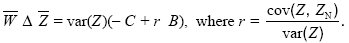
We see that the coefficient r is the ratio between the covariance between the individual and its neighbors and the variance across individuals. (We are focusing on breeding values, and so these are the additive genetic covariance and variance; p. 393.) Now, this ratio is just the regression coefficient, which predicts the mean in the neighbors, given the value of the individual. (Given that an individual has trait value Z, the expected value of Z_N is + r(Z – ).) It is this regression coefficient that determines the strength of kin selection (see Fig. WN21.5).

As we explain on pages 601–602, individuals that interact with each other may be genetically similar for a variety of reasons. The most important is that they are related; that is, they carry genes that are identical by descent. To see how to calculate the regression coefficient r from probability of identity by descent, F, consider the effects of a single gene in a diploid individual and one of its neighbors. The effects of the two genes on the focal individual are Z = X + X^*, and the effects of the two genes in the neighbor are Z_N = X_N + X^*_N (see Fig. WN21.6). The variance of the individual is var(Z) = var(X + X^*) = var(X) + 2cov(X, X^*) + var(X^*). Now, the variance of a randomly chosen gene from the population is by definition half the additive genetic variance, var(X) = var(X^*) = V_A/2. The covariance between the two gene copies from the same individual is the chance that those genes are identical by descent (F) times the variance of effect of their ancestor, which is again V_A/2. Thus, var(Z) = V_A(1 + F). The covariance between the values in the individual and its neighbor is the sum of the covariances of effects of the four pairs of genes:

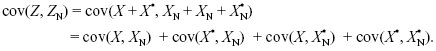
By the same arguments as before, this is 4 × F_N × (V_A/2) = 2F_NV_A, where F_N is the probability of identity by descent between a gene in the focal individual and a gene in the neighbor. Putting all this together, we find the relationship between r and F, F_N: