Evolution Chapter 23 Answers
|
Answer 23.1
|
| i) |
Deleterious mutations reduce the average fitness by exp(–U) NOTE 23F Therefore, the overall fitness is exp(–U)(1 – exp(–2U)). This has a maximum of 0.38 at U = 0.55. This can be found most easily from the graph (red curve in Fig. P23.3). Alternatively, the maximum occurs where the derivative of exp(–U)(1 – exp(–2U)) with respect to U is zero. Differentiating with respect to U, –exp(–U) + 3exp(–3U) = 0, so 3 = exp(2U) or U = (1/2)loge(3) = 0.55.
|
| ii) |
Think about an allele that increases the genome-wide mutation rate from U to U*. Such an allele gains a reduction in the cost of repairing damage, from (1 – exp(–2U)) to (1 – exp(–2U*)). Although it is increasing from low frequency, it will only stay associated with the mutations that it causes on its own chromosome; the other nine chromosome pairs will have a mutation load determined by the original mutation rate U. So, the net mutation load of such an allele is exp(–U*/10 – 9U/10), compared with exp(–U) for the competing allele. Thus, its net fitness is exp(–U/10)(1 – exp(–2U)). Alleles will be able to invade if they increase this function, and so the population will evolve toward a maximum fitness of 0.21 at U = 1.52 (right arrow in Fig. P23.3). Fitness is much lower than the optimum for the whole individual.
|
|
Answer 23.2
|
| i) |
In a mutation-selection balance, the expected number of deleterious mutations is U/s = 0.002/0.02 = 0.1. Assuming multiplicative effects, the number carried by each individual will follow a Poisson distribution around this average, with a proportion exp(–U/s) = 0.905 carrying no deleterious mutations. The mean fitness is exp(–U) = 0.998 (pp. 539 and 552).
|
| ii) |
Mutation-free individuals have a fitness 1/exp(–U) = exp(+U) greater than the average for the whole population. Because the latter must be 1 for a steady population size, the absolute fitness of a mutation-free individual must be exp(U) = 1.002.
|
| iii) |
Assuming that the actual number of mutations produced follows a Poisson distribution, with an expectation of U* = 0.2, the chance that an offspring has no mutations is exp(–U*) = 0.819. To see this, suppose that there is a low rate of mutation μ at a large number n of loci. Then, the chance that none of them mutate is (1 – μ)n ~ exp(–nμ) = exp(–U); see Chapter 28).
|
| iv) |
In the next generation, an individual carrying the mutator allele is expected to produce a fraction exp(–U*) = 0.819 mutation-free offspring. From ii), the absolute number of offspring is exp(+U) = 1.002, and so the expected number of mutation-free offspring is exp(–(U*–U)) = 0.820. After t generations, the expected number is exp(–(U* – U))t = exp(–(U* – U)t).
|
| v) |
Summing over all future generations, we expect a total of 1 + 0.820 + 0.8202 + ··· ~5.57. If we approximated to continuous time, we would have
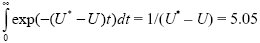
mutation-free offspring. This is a reasonably good approximation, because changes between generations are not too large.
|
| vi) |
The fittest class makes up exp(–U/s) = 0.905 of the population. So, there are exp(–U/s)N individuals in the fittest class that can mutate, and the rate of mutation to give favorable alleles in the fittest class is exp(–U/s)Nμ = 0.905 × 107 × 10–10 = 0.905 × 10⁻³ per generation.
|
| vii) |
There is a chance exp(–U/s) that the mutator allele will arise on the fittest background; if it does so, then from v), we expect a total of about 1/(U* – U) mutator alleles to be produced on the fittest background, and the favorable allele arises at a rate (U*/U)μ in these. Therefore, each mutator allele produces successful favorable mutations at a rate (U*/U)μ exp(–U/s)/(U* – U). For U* >> U, this is approximately μ exp(–U/s)/U. The relative advantage of the mutator alleles over the nonmutators is about 1/U or, in this example, about fivefold. Favorable mutations are five times as likely to be established with the mutator alleles, and so the mutator alleles gain a fivefold greater chance of being swept to fixation.
|
| viii) |
If the favorable mutation does arise with a mutator allele, it will soon acquire an extra mutation load and be eliminated along with the mutator allele. The number of mutation-free offspring, even with the favorable allele, would be just (1 + s*)exp(–(U* – U)) ~0.829, and so the mutation-free class would still decline. If the favorable allele had a larger advantage, then it could increase even if associated with deleterious mutations. However, it would then fix those deleterious mutations as it swept to fixation itself.
This example shows how inefficient selection is when there is no recombination: Weakly favorable alleles cannot fix unless they are in backgrounds free of deleterious mutations, and strongly favored alleles are liable to fix deleterious alleles inadvertently. Mutator alleles generally do not aid adaptation, because they generate far more deleterious alleles than favorable ones. NOTE 23G
|
|
Answer 23.3
|
| i) |
In a stable sexual population, with an equal sex ratio, each female produces two offspring on average. If these offspring are genetically identical to their mother, then the parthenogenetic type will double in frequency in every generation. NOTE 23H
|
| ii) |
Initially, males will mate with parthenogenetic females and help rear their daughters. Parthenogenetic females will be selected to attract mates, because they gain considerable parental care, but males will be under strong selection to avoid parthenogenetic females. If the selection on males is effective, parthenogenetic females will lose parental care and produce only 2 × (1/4) as many offspring and so become extinct. NOTE 23I
|
|
Answer 23.4
|
| i) |
Each selfing plant produces on average one seed. Each heterozygote will produce on average 1/4 wild-type homozygotes, 1/2 heterozygotes, and 1/4 selfing homozygotes. Thus, the number of heterozygotes decreases by 1/2 every generation, and eventually these die out. However, an average of 1/4 + (1/4 × 1/2) + ··· = 1/2 selfing homozygote will be produced from each heterozygote. These selfing homozygotes breed true and so, on average, persist at the same frequency. Ultimately, however, they will die out by chance. NOTE 23J Writing out the recursion more formally:
|
| ii) |
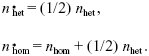
If selfing plants also continue to each fertilize one other seed, on average, then they must increase on average. Each heterozygous plant now fertilizes a wild-type seed, and so on average produces 1/2 a heterozygote. Each homozygous plant now fertilizes a wild-type seed and produces one other heterozygote. Adding these contributions to the previous recursion:
We can follow the numbers through successive generations, starting with one heterozygote: {1,0}, {1, 1/4}, {1 1/4, 1/2}, ... (Fig. P23.4). This shows that after a few generations, the numbers increase by a factor 3/2 per generation, with twice as many heterozygotes as homozygotes.
To see this algebraically, we look for a solution where nhet = a nhom, and where numbers increase by λ each generation (Chapter 28):
λ a nhom = a nhom + nhom,
λ nhom = nhom + (a/4) nhom.
Canceling nhom,
λ a = (1 + a),
λ = (1 + a/4).
This has the solution λ = 3/2, a = 2 (which can be obtained graphically or by solving a quadratic equation).
|
|
Answer 23.5
|
| i) |
Over the whole population, NU = 1 mutations arise per generation, on average (where N = 109 is the number of haploid individuals, and U = 10–9 is the total rate of mutation per genome per generation). The chance that each mutation will fix is approximately 2s = 2 × 0.05 = 0.1 (p. 490), and so, on average, we will expect to wait ten generations before such an allele starts to increase.
|
| ii) |
The ratio of allele frequencies is initially p/q = 10–9, and increases by a factor 1 + s = 1.05 in each generation. So, allele frequencies will be equal (p = q = 1/2) when 10–9 (1.05)t = 1, or t = log(109)/log(1.05) ~ log(109)/0.05 ~ 420 generations (pp. 468–469; Box 17.1). NOTE 23K
|
| iii) |
We therefore expect about 42 other beneficial alleles to become established while the first one is still rising from low frequency.
|
| iv) |
Crucially, if there is no recombination, then only 1 of the approximately 43 competing alleles can actually fix (see Fig. 23.18). (If the alleles all had identical fitnesses, they would then persist together for a while, until one fixed by chance. But if the selection coefficients vary, then the fittest one will eventually fix, even though the others would have given an additional fitness advantage if they could have been brought together in the same genome.) The rate of substitution is therefore approximately 1 every 420 generations, because the alleles have to fix in series.
|
| v) |
In a sexual population, with free recombination, the rate would be 1 in 10 generations, about 42 times greater.
|
| vi) |
By this argument, the rate of substitution in a sexual population is approximately 2sNU and in an asexual population, ~ 1/((1/s)log(N)) for a haploid population of N genes. Therefore, the relative advantage of sex is 2NU log(N), which increases with increasing N. This advantage does not arise in a very small population, because, in that case, beneficial alleles arise so rarely that they do not interfere with each other. However, when the population is large enough that many beneficial mutations arise in each generation (NU >> 1), as is assumed here, only a small fraction can survive in an asexual population, and so sex has a large advantage. NOTE 23L
|
|
Answer 23.6
|
| i) |
The chance that one of the four genes (two in the mother and two in the father) is a rare allele, at frequency p, is 4p. In this case, one of the parents will be a heterozygote and half the offspring will be heterozygotes. If competition is intense, then all the survivors will be heterozygotes and the allele frequency will be 1/2. Overall, then, the expected frequency among the survivors is (1/2)4p = 2p, and we expect the allele frequency to double in every generation.
|
| ii) |
If the female mates with two males, then the chance that one of the six genes that contribute to the family carries allele P is 6p. By the same argument as before, the allele frequency among emerging individuals is 3p, and the allele increases threefold in every generation. NOTE 23M
|
|
Answer 23.7
|
| i) |
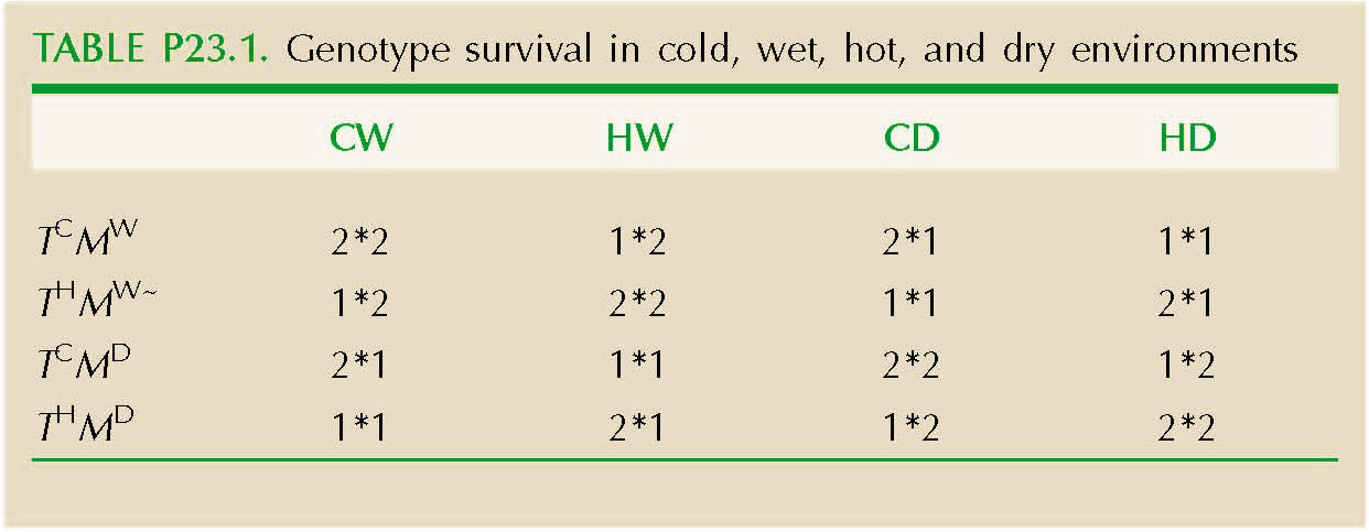
Table P23.1 shows the relative survival of each genotype (rows), in each environment (columns).
To work out what happens to a rare TH allele introduced at low frequency p into a TCMW population, we look at its relative survival in each of the four environments. Comparing the top two rows, we see that it has half the survival in cold patches, and so its frequency falls to p/2 (assuming p << 1). In hot patches, it has twice the survival, and so its frequency increases to 2p. Since hot and cold patches are equally frequent, on average its frequency increases to (3/2)p. Similarly, the TC allele would increase in a population nearly fixed for TH, and by symmetry, there will be a stable equilibrium at p = 1/2.
Once this polymorphism for TH, TC is established, in a population still fixed for MW, the average survival in wet patches is 3, and in dry patches, 3/2. Then, an MD allele will have relative fitness (3/2)/3 = 1/2 in wet patches, and 3/(3/2) = 2 in dry patches (compare the averages of the first two rows and the average of last two rows). So, MD will invade an MW population, and there will be a stable polymorphism at equal allele frequencies for both loci. NOTE 23N
|
| ii) |
At equilibrium, equal proportions of every genotype enter the breeding pool, and so there is no linkage disequilibrium. Therefore, recombination has no effect on the population, and there is no selection for higher or lower recombination (pp. 669–671).
|
| iii) |
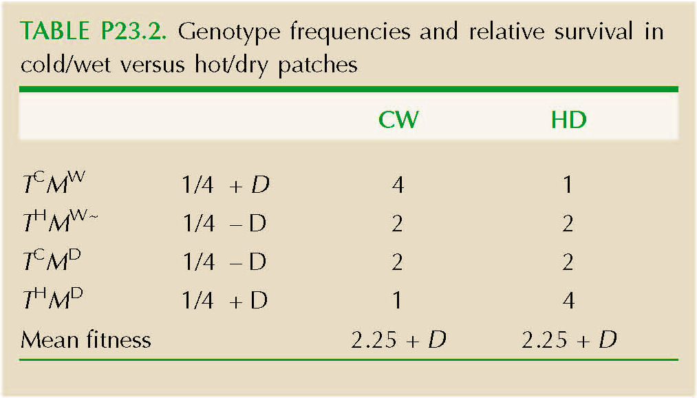
The same arguments as in i), and the symmetry of the problem, show that there will still be a stable equilibrium with equal allele frequencies at both loci. However, there will now be linkage disequilibrium, with an excess of TCMW and THMD. Write the frequencies of each of these genotypes among newborn individuals as (1/4 + D) and of the other two as (1/4 – D). The genotype frequencies and relative survival in each patch are shown in Table P23.2.
The genotype frequencies emerging from a CW patch are in the proportions (4(1/4 + D), 2(1/4 – D), 2(1/4 – D), (1/4 + D)). The frequencies emerging from a HW patch are the same, but in reverse order, and so the overall frequency is ((5/2)(1/4 + D), 2(1/4 – D), 2(1/4 + D), 5/2(1/4 + D)), divided by the total, (2.25 + D). Allele frequencies remain 1/2, but linkage disequilibrium has increased. Writing the first genotype frequency as 1/4 + D*, we find that D* = (1 + 36D)/4(9 + 4D). With no recombination, this would increase until D reaches its maximum of 1/4. However, if loci are unlinked and mating is random, then D decreases by a factor of one-half in each generation. At equilibrium, then,
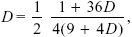
and so D = 0.027. This can be found by drawing a graph of the formula or by solving a quadratic equation. This is about one-tenth of the maximum value (D = 0.25); genotype frequencies at the beginning of the generation are 0.277:0.223:0.223:0.277.
|
| iv) |
The average fitness within each patch,  = 2.25 + D, increases with the strength of linkage disequilibrium, because the increase in the fittest genotype (fitness 4) outweighs the increase in the least fit (fitness 1). If only TCMW and THMD were present (D = 1/4), then mean fitness would be (4 + 1)/2 = 2.5, compared with (4 + 2 + 2 + 1)/4 = 2.25 if D = 0. This suggests that selection will act against recombination, but it is not reliable evidence, since it is based on population rather than individual fitness. = 2.25 + D, increases with the strength of linkage disequilibrium, because the increase in the fittest genotype (fitness 4) outweighs the increase in the least fit (fitness 1). If only TCMW and THMD were present (D = 1/4), then mean fitness would be (4 + 1)/2 = 2.5, compared with (4 + 2 + 2 + 1)/4 = 2.25 if D = 0. This suggests that selection will act against recombination, but it is not reliable evidence, since it is based on population rather than individual fitness.
|
| v) |
Now we know that in one generation, when environments CW and HD are present, the average fitnesses of the four genotypes are {5/2, 2, 2, 5/2}. In the next generation, when CD and HW are present, the average fitnesses will be {2, 5/2, 5/2, 2}. Write the genotype frequencies at the start of the two-generation cycle as {1/4 – D, 1/4 + D, 1/4 + D, 1/4 – D}. The association must increase under selection for a positive association to +2D, then halve to +D at the beginning of the next generation, immediately after random mating, decrease to –2D under selection for the opposite association, and finally halve to –D to start the two-generation cycle again. We therefore have the formula +2D = (1 – 36D)/4(9 – 4D), where we have replaced +D by –D in the previous formula for the effect of selection on D. This gives D = 0.0093, which is a weaker association, because selection alternates in direction.
The average fitness is now just (2.25 – D) in each generation, because linkage disequilibrium tends to be in a direction opposite to that favored by selection. This suggests that increased recombination will be favored. However, this is again not a reliable argument. Ideally, one would follow the frequency of a modifier allele that alters the rate of recombination and that may gain an indirect advantage by tending to produce fitter offspring.
|
|
Answer 23.8
|
| i) |
The variance of the midparental values is half the variance of the parental values. Adding the within-family variance Vf we have that  = (1/2)Vg + Vf. = (1/2)Vg + Vf.
|
| ii) |
Therefore, at equilibrium, Vg = 2Vf.
|
| iii) |
The mean fitness is approximately given by the average of 1 – z2/2Vs. Because the average of z2 is Vg, this is just 1 – Vg/2Vs.
|
| iv) |
The probability of finding a trait value z after selection is just the initial distribution multiplied by the relative fitness. Using the formula for the normal distribution (Chapter 28) this is proportional to
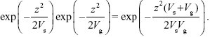
Therefore, the variance of the selected population is VsVg/(Vs + Vg), which is lower than Vg.
|
| v) |
Using the same argument as before, we have that
At equilibrium, = Vg. This leads to a quadratic equation with solution
For example, with Vs = 10Vf, Vg = 1.74Vf at equilibrium (Fig. P23.5). (This genetic variance is measured in newborns, immediately before selection; top line in Fig. P23.5.) Stabilizing selection has reduced Vg from 2Vf to 1.73Vf.
|
| vi) |
We know that the change in mean caused by a selection gradient β is just βVg (p. 478). So, the mean changes at a rate proportional to the equilibrium genetic variance calculated above, a value reduced somewhat below 2Vf by stabilizing selection. Moreover, directional selection of this form shifts the mean but does not alter the variance of the trait. This can be verified by using the same method as in iv). So, the mean responds to selection at a constant rate. NOTE 23O
|
| vii) |
With asexual reproduction, each individual produces identical offspring. Therefore, stabilizing selection rapidly reduces variation, so that eventually, only the fittest genotype remains. If we ignore directional selection, then after one round of selection, the variance has decreased to VsVg/(Vs + Vg). A little algebra shows that after t rounds of selection, it has decreased to VsVg/(Vs + t Vg). For example, with Vs = 5Vg, the genetic variance has halved after five generations, and decreased to 10% of its original value after 45 generations. If selection is purely stabilizing, then asexual reproduction gives higher mean fitness, because only the best genotype is present: There is no load due to variation around the optimum. However, if directional selection also acts, then the population can respond much faster with sexual reproduction and, in the long run, will have higher mean fitness. This population-level advantage corresponds to an individual advantage to modifier alleles that increase sex and recombination.
In terms of the discussion on pages 674–676, stabilizing selection generates negative linkage disequilibria among the underlying alleles, which impede the response to selection; sex and recombination break these up.
|
|
Answer 23.9
|
| i) |
The expected fitness in the next generation is just 1 + δ/2. This is because the gene has a chance of 1/2 of staying with each unlinked gene that gives it an advantage, and a chance 1/2 of recombining away and return to an average genetic background. The expected fitness in successive generations is 1 + δ, 1 + δ/2, 1 + δ/4, ... .
|
| ii) |
The expected total number of copies is (1 + δ)(1 + δ/2)(1 + δ/4) ···, which is approximately 1 + δ + (δ/2) + (δ/4) + ··· = 1 + 2δ for small δ.
|
| iii) |
If the ultimate number of copies left by a gene with present fitness 1 + δ is 1 + 2δ, then the variance in this ultimate number is E[(2δ)2] = 4E[δ2] = 4v. The rate of drift is therefore (4v/2N)pq, which is four times the rate due to noninherited variance in fitness.
|
| iv) |
The inherited component of fitness variance is vi = 0.2 × 1.25 = 0.25, and the noninherited (“environmental”) component is ve = 0.8 × 1.25 = 1. So, the total rate of drift is (ve + 4vi)(pq/2N) = 2(pq/2N). The effective population size is therefore halved: Ne/N = 1/2.
|
| v) |
The chance that a favorable allele will be fixed is halved by this inherited component of fitness variance.
|
|
Answer 23.10
|
| i) |
The mean fitness is exp(–U) = exp(–2) = 0.135.
|
| ii) |
If the effects of different mutations multiply together, then there is no linkage disequilibrium, and recombination has no effect (p. 552 and pp. 669–672). Therefore, the mean fitness is again 0.135.
|
| iii) |
The change in relative fitness is
Therefore, the expected total number of deleterious mutations at equilibrium is expected to be U/s = 200, which is consistent with the initial assumption.
|
| iv) |
The distribution will be approximately Poisson and so will have a variance equal to the mean (Fig. P23.6); the standard deviation is  = 14.1. NOTE 23P = 14.1. NOTE 23P
|
| v) |
The mean fitness is
This is much higher than that of an asexual population.
|
|
Answer 23.11
|
| i) |
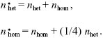
Each female heterozygous for the new allele (Aa, say) will produce on average one haploid male; half of these will carry A. They will also produce one daughter, fertilized by an aa male, and so half of these will be Aa. Haploid males will produce one Aa female, and one Aa son. Finally, diploid Aa sons will produce on average 1/2 an Aa daughter and 1/2 a diploid Aa son. So, if we write the numbers of these three types as nf, nhm, ndm, we have
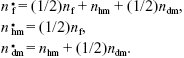
Iterating through the generations, starting with a heterozygous female, the numbers of heterozygous females, haploid males, and heterozygous diploid males are

See Figure P23.7. Eventually, this settles to a steady state of increase, by a factor λ = 1.21 each generation. NOTE 23Q
|
| ii) |
In the original population, we assume that selection acts mainly against heterozygotes, so that the frequency of deleterious mutations at each locus is μ/s << 1. Therefore, the chance that a haploid male does not carry a recessive lethal at any of n loci is (1 – μ/s)n ~ exp(–nμ/s). Because the total mutation rate per diploid genome is U = 2nμ = 0.2, the chance that the male survives, with no recessive lethal, is exp(–U/2s) = exp(–0.2/(2 × 0.02)) = exp(–5) = 0.0067. (We could also get this result by seeing that the number of lethals is Poisson distributed with expectation 2U/s = 5, and so the chance of having none is exp(–5).) Thus, if haploid males were produced, they would almost all die because recessive lethals are unmasked. This makes it likely that haplodiploidy will evolve only in inbred populations that have purged deleterious recessive alleles.
|
| iii) |
Males cannot carry any recessive lethals, but they may be present in heterozygous females. Suppose that females carry an expected number n of recessive lethals as heterozygotes. Then, they will pass on an average of n/2 to their daughters. New mutations will add U to each daughter’s diploid genome, and so at equilibrium, we have n = U + n/2, or n = 2U. Thus, we expect each daughter to inherit U recessive lethal alleles from her mother and acquire U new ones.
The load on the population will be borne entirely by males. These will acquire an average of n/2 = U recessive lethal alleles from their mother, and U/2 new ones by mutation in their haploid genome. Therefore, the chance that they will survive, without getting any recessive lethals, is exp(–3U/2); for U = 0.2, this is 0.74. Thus, if haplodiploidy could be established, it would not lead to excessive load, because recessive alleles would be eliminated by selection on haploid males.
|
|
Answer 23.12
|
| i) |
Overall fitness is proportional to (A/m)(2m)k, so we expect fitness to increase with gamete size, when k > 1.
|
| ii) |
Suppose that the population is fixed for the maximum gamete size, M; mean fitness will be (A/M)(2M)k. A new type, with gametes of size m << M, will have fitness (A/m)(M + m)k ~ (A/m)Mk. Its relative fitness is M/2km, and so it will increase if m is small enough.
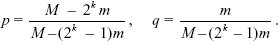
|
| iii) |
Suppose that there is a frequency p of very small gametes (m << M) and q of very large gametes. A small gamete has a chance p of meeting another small one, in which case the zygote cannot survive. It has a chance q of meeting a large gamete, giving survival (M + m)k ~Mk. Because A/m are produced, the net fitness of a small gamete is q(A/m)Mk. A large gamete has a chance p of meeting a small gamete, giving survival ~Mk, and q of meeting another large one, giving survival (2M)k. Overall, then, their fitness is (A/M)(p + q 2k)Mk. At equilibrium, the fitnesses of the two kinds of gametes must be the same, and so we find that
For m << 2–kM, this implies that mostly very small gametes will be produced, even though the population as a whole would be better off if large gametes were produced. Of course, once different gamete sizes are established, different mating types will evolve in order to avoid inbreeding depression (p. 686); then, gametes no longer mate at random, as assumed here.
|
|
Answer 23.13
|
| i) |
The optimal value of E can be found by sketching a graph of net fitness, that is, [E X/(E + X)] exp(–βE), for given βX. More generally, we can differentiate with respect to E and set the slope to zero, which leads to the solution
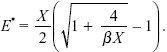
When the cost of enzyme production is low (βX = 0.01), enzyme concentration is high relative to the substrate (E*/X = 9.5; red dot in Fig. P23.8); when the cost is high (βX = 0.5), enzyme concentration equals substrate concentration (E*/X = 1; blue dot in Fig. P23.8).
|
| ii) |
Figure P23.9 shows the fitness as a function of enzyme concentration, assuming that the production cost is held fixed. The red dots show the heterozygote and homozygote enzyme concentrations when E* is optimal for a low cost (βX = 0.01); then, the heterozygote has 91% the fitness of the homozygote, so that the loss-of-function allele is almost recessive. The blue dots show the case where E* is optimal for a high cost (βX = 0.5); then, the heterozygote has 67% the fitness of the homozygote, and so the loss-of-function allele is roughly additive.
|
References
André J.B. and Godelle B. 2006. The evolution of mutation rate in finite asexual populations. Genetics 172: 611–626.
Crow J.F. and Kimura M. 1965. Evolution in sexual and asexual populations. Am. Nat. 99: 439–450.
Crow J.F. and Kimura M. 1969. Evolution in sexual and asexual populations: A reply. Am. Nat. 103: 89–91.
Maynard Smith J. 1968. “Haldane’s dilemma” and the rate of evolution. Nature 219: 1114–1116.
Maynard Smith J. 1974. Recombination and the rate of evolution. Genetics 78: 299–304.
Sniegowski P., Gerrish P.J., and Johnson T. 2000. Evolution of mutation rates: Separating causes from consequences. BioEssays 22: 1057–1066.
|


