Evolution of Female Preferences

The different ways in which female preferences may evolve can be illustrated using a simple model, which was first analyzed by Lande (1981). Males express a quantitative trait (e.g., tail length), which is under stabilizing selection, so there is an optimal value (Fig. WN20.10, dashed horizontal line) for which male survival is greatest (right box). Sexual selection also acts on the trait, through a female mating preference. Each female prefers a certain trait value, and this preferred value varies as a second quantitative trait. Thus, the population can be described by the mean values of the male trait and the female preference (Fig. WN20.10, square boxes).

To begin with, assume that there is no direct selection on the female preference—that is, female fitness does not depend on what kind of males they prefer (Fig. WN20.10, top box). Now, there are many possible equilibria. If females prefer the trait that maximizes male survival, then natural and sexual selection coincide, and the population will evolve toward the optimum (Fig. WN20.10, open circle). However, if females prefer a larger trait value, then there will be an equilibrium in which natural and sexual selection counterbalance; males will then have lower survival than they might. There is a line of equilibria, which represents different balances between natural and sexual selection (Fig. WN20.10, diagonal lines).

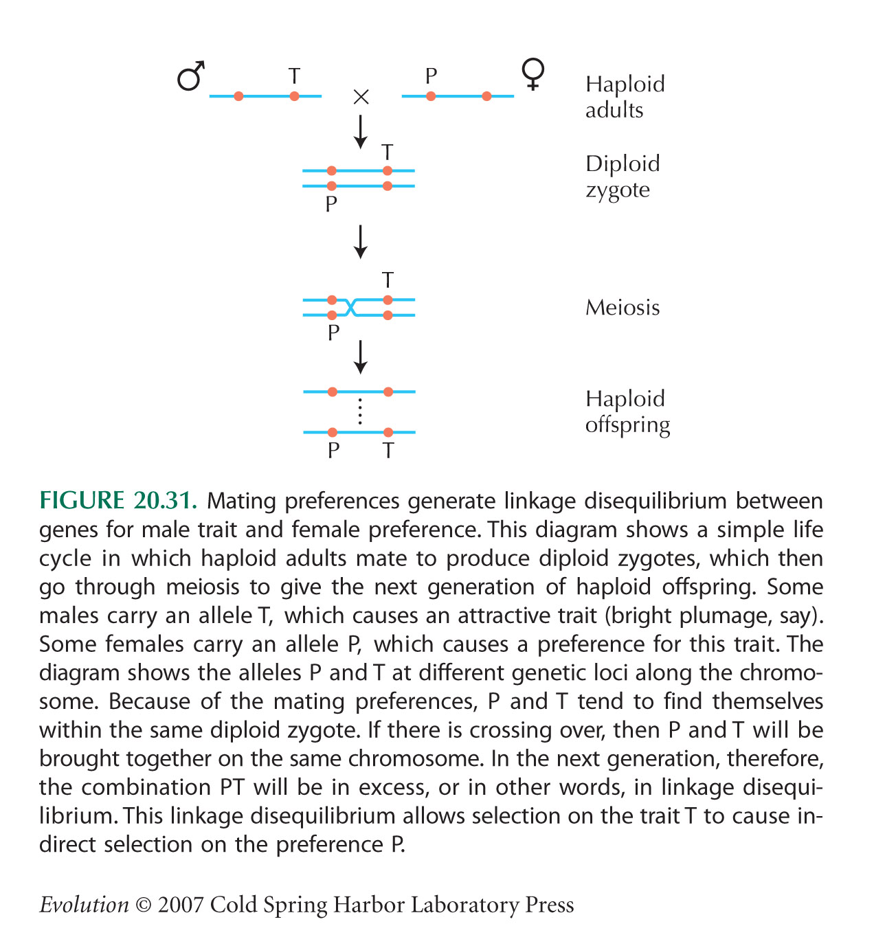
Mating preferences generate a genetic correlation between male trait and female preference. (The argument for quantitative traits is the same as for discrete genes; Fig. 20.31.) Therefore, as the mean male trait increases, the mean female preference will also increase by indirect selection. (This is an example of hitchhiking; p. 485.) Populations evolve along diagonal lines, which have a slope that depends on the strength of the genetic correlation (arrows in Fig. WN20.10). If the genetic correlation is strong, then a small change in the trait will lead to a large shift in preference, and so the population will evolve along diagonal lines that are close to horizontal (Fig. WN20.10A). These lines do not intersect with the line of equilibria, and so that line is unstable. The population will evolve trait and preference combinations that become more and more exaggerated. This is Fisher’s runaway process.

The genetic correlation between trait and preference is more likely to be weak. Then, the population will evolve toward the line of equilibria (Fig. WN20.10B) and will reach a balance between natural and sexual selection. Whether the trait is close to the optimum favored by natural selection on male survival or instead an exaggerated trait is maintained by an extreme female preference depends on the arbitrary sensory biases of the female.

If even slight selection acts directly on the female preference (Fig. WN20.10C, top), then the population will evolve along the line of equilibria to whatever preference maximizes the females’ immediate fitness. In general, the preferred trait will not maximize male survival, so that sexual selection will be maladaptive.