Evolution Chapter 22 Answers
|
Answer 22.1
|
| i) |
It is simplest to think about this from the point of view of this rare allele. It has a 10% chance of finding itself in an F1 hybrid, in which case its bearer will die young, rather than being sterile. Therefore, an extra individual will emerge from the patch instead and that extra individual has a 50% chance of carrying the allele in question. This kin selection gives this allele an advantage of 5% over the alternative allele.
|
| ii) |
Now, the allele gains half the advantage, or 2.5%: If it is inherited through the mother, it has the same chance of being found in a sibling, whereas if it is inherited through one of the many fathers, it is unrelated to its siblings.
|
|
Answer 22.2
|
| i) |
The chance that a lineages crosses, per generation, is m, and so the chance that a lineage does not cross in T generations is (1 – m)T ~ exp(–mT) (Chapter 28). In this case, m = 5 × 10⁻⁷ and T = 106, and so each lineage has a chance of only ~exp(–0.5) = 0.61 of tracing back without crossing into the other species. The chance that neither jumps across is only ~ 0.612 = 0.37. Thus, even a very low migration rate can lead to substantial gene exchange over long times. The expected time to coalescence, given that there has been no gene flow, is T + 2Ne = 1.2 × 10⁶ generations.
|
| ii) |
The chance that one lineage crosses, but the other does not, is approximately exp(–mT)(1 – exp(–mT)) = 0.24. Because one or the other lineage could jump across, the total probability is 2 × 0.24 = 0.48. Now, the two lineages can coalesce at a rate 1/2Ne per generation. If there are t generations remaining before the ancestral population is reached, then the chance that there will not be a coalescence in this time is ~exp(–t/2Ne). As a rough approximation, we can take the jump to occur halfway back (i.e., t = T/2), on average. Therefore, the chance that the lineages jump into the same population, yet do not coalesce, is 0.48 × exp(–T/4Ne) = 0.48 × 0.082 = 0.039. This is quite small, because Ne << T, and so once two lineages are in the same population, they are likely to coalesce before they get back to the ancestral population.
|
| iii) |
The chance that a lineage jumps within τ = 105 generations is approximately mτ = 0.05. The chance that one or the other jumps is therefore 2mτ(1 – mτ) ~ 0.10. (We do not count the small chance that both jump, and we ignore multiple crossings, making the same approximation as in 2ii).) Once the two lineages are within the same species, they have probability (1 – 1/2Ne)t ~ exp(–t/2Ne) of not coalescing in t generations; the chance that they do coalesce is thus 1 – exp(–t/2Ne). The time t available for coalescence will be uniformly distributed between 0 and τ = 105 generations. As a simple approximation, we can take it to be τ/2 = 0.5 × 10⁵ generations, giving a net chance of coalescence of 2mτ(1 – mτ)(1 – exp(–τ/4Ne)) = 0.021.
|
| iv) |
Extending the argument given in iii), the chance that the two lineages cross into the same population, and then coalesce by time τ, is 2mτ(1 – mτ)(1 – exp(–τ/4Ne)), for τ < T. The chance that they do not coalesce in this time is 2mτ(1 – mτ)(1 – exp(–τ/4Ne)). For times earlier than the divergence time T = 106 generations (i.e., for τ > T), the chance that they do not coalesce is approximately (1 – 2mT(1 – mT)(1 – exp(–T4Ne))exp(–(τ – T)/(2Ne)). This is shown by the red line in Figure P22.3; it is close to the exact calculation (blue line in Fig. P22.3), which takes into account multiple crossings. There is a rapid acceleration of coalescence for times earlier than T = 106 generations, when the populations join in a single ancestral population; but, nevertheless, the mean coalescence time is ~860,000 generations, which is less than T. NOTE 22G
|
|
Answer 22.3
|
| i) |
First, there are more sites unique to gorilla than to either chimpanzee or human, indicating that gorillas have been evolving separately for longer than either humans or chimpanzees. Second, the numbers of sites in classes H and C and in classes HG and CG are very similar, which is consistent with H and C being the youngest clade. Finally, sites such as HG or CG (which imply that the genealogy must be different from the phylogeny) are much less common than sites in the class HC.
|
| ii) |
The number of sites that are different between humans and chimpanzees are the sum of classes H, C, HG, CG. Thus,
H vs. C H + C + HG + CG 58,196
H vs. G H + G + HC + CG 75,360
C vs. G C + G + HC + HG 75,224.
The expected time to coalescence of a lineage from human and a lineage from chimpanzee is T0 + 2Ne (because it takes 2Ne generations for two lineages within the same population to coalesce). For either human or chimpanzee lineages to coalesce with a gorilla lineage is expected to take an additional T1 generations. The difference between the average divergence of human or chimpanzee from gorilla, and human from chimpanzee, is 75,292 – 58,196 = 17,096 sites, out of a total length L = 9.3 Mb. This fraction of divergence is expected to equal 2μT1. Therefore, we estimate T1 = 92,000 generations.
|
| iii) |
The rate of coalescence of the two lineages (H, C) is 1/2Ne per generation. So, the chance that they do not coalesce during T1 generations is (1 – 1/2Ne)T1 ~ exp(–T1/2Ne). If they do not coalesce, then there will be three lineages in the population ancestral to human, chimpanzee, and gorilla, and three ways for them to coalesce (H with C first, or H with G, or C with G). Thus, overall, the chance that the first coalescence is either H with G or C with G, so that the genealogy differs from the phylogeny, is (2/3)exp(–T1/2Ne).
|
| iv) |
The expected number of sites in class CG or HG depends on the expected length of the corresponding branch. There is a chance (1/3)exp(–T1/2Ne) that the first coalescence is C with G; then, it takes on average a further 2Ne generations for the branch ancestral to (C, G) to coalesce with the human lineage. Thus, the expected number of CG sites is μL × 2Ne × (1/3)exp(–T1/2Ne), and similarly for HG sites.
|
| v) |
We can therefore estimate that (866 + 993) = μL × 2Ne × (1/3)exp(–T1/2Ne). Substituting for μL = 9,300,000 × 10–8 = 0.093 and T1 = 92,000 we have an equation for Ne. This can most easily be solved by drawing a graph of μL × 2Ne × (1/3)exp(–T1/2Ne) against Ne; we estimate Ne ~ 36,000. The chance that a genealogy is discordant is (2/3)exp(–T1/2Ne) ~ 18.5%. The time back to the split between human and chimpanzee can be estimated from the human–chimpanzee divergence. From ii), we have that 58,196 = 2 μL(T0 + 2Ne), and so T0 ~ 240,000 generations (6 Mya if we assume 25 years per generation). NOTE 22H
|
|
Answer 22.4
|
| i) |
There have been 2000 substitutions in each autosomal genome, and so (assuming that the same substitution never occurs in the two lineages) there are 2000 × 2000 pairs that might be incompatible. If a fraction p = 10–3 of pairs are incompatible, that gives 4000 incompatibilities. However, only incompatibilities that involve two dominant alleles can be expressed in the F1. 1% of alleles are dominant, and so only a fraction, 0.012 = 0.0001, of pairs will involve dominant alleles. Overall, then, we expect about 0.4 pairs of recessive alleles that express an incompatibility in the F1, and we expect fitness to be reduced by, on average, a factor (1 – s)0.4 = 0.96. NOTE 22I
|
| ii) |
An F1 female will inherit an X from the father and an X from the mother; incompatibilities on the X will behave in the same way as for incompatibilities on the autosomes, and so, again, only recessive × recessive incompatibilities can be expressed. Using the same argument as in i), the fitness of F1 females is reduced by ~2500 × 2500 × 10–3 × 0.012 ~ 0.625 incompatibilities, which reduce fitness by (on average) ~ (1 – s)0.625 = 0.936.
|
| iii) |
In F1 males, only a single X is inherited from the mother, and so there can be no incompatibility between genes on the X. Dominant × dominant incompatibilities will be expressed whether they are on the X or the autosomes and will reduce fitness by 0.936 as in ii). However, recessive alleles on the X can interact with dominant alleles on the autosomes, contributing another 2000 × 0.01 × 500 × 0.99 × 10–3 = 9.9 incompatibilities, and reducing fitness by ~0.936 × 0.99.9 = 0.33. This much lower fitness of F1 males compared with F1 females is consistent with Haldane’s rule.
|
| iv) |
The fitness of an F1 female is (1 – s)n2pα2, where n is the number of substitutions and the fitness of an F1 male is (1 – s)n2p(α2 + χ(1−χ)α(1 − α)). Both of these decrease as an approximately Gaussian curve, of the form exp(–n2/(2v)), where v is the variance. However, F1 male fitness decreases much faster. (See Fig. P22.4.) NOTE 22J
|
| v) |
First, consider autosomal × autosomal incompatibilities. We expect 200 × 200 × 10–3 = 40 of these. If both the alleles involved are recessive (probability (1 – α)2 ~ 0.98, then only the double homozygote will suffer in the F2: assuming no linkage, these will be 1/16 of the F2 population. If one is recessive and one dominant (probability 2α(1 – α) ~ 0.04), then 3/16 will suffer, and if both are dominant (probability 0.0001), 9/16. Overall, then, an average of (0.98 + 0.04 × 3 + 0.0001 × 9)/16 = 0.065 of the F2 will suffer, and the net fitness will be ~(1 – 0.065s)40 = 0.770: We expect the F2 to have significantly lower fitness than the F1, mainly because of the cumulative effects of large numbers of recessive × recessive incompatibilities.
For females, the effects of X-linked incompatibilities are exactly the same (for simplicity, we neglect linkage). Allowing for a total of 250 × 250 × 10–3 = 62.5 incompatibilities gives a still tinier fitness in the F2, of (1 – 0.065s)62.5 = 0.665. Males carry only a single X, and so in the F2, alleles segregate at frequencies 1/2:1/2. Therefore, autosomal × X-linked incompatibilities will be expressed in 1/8 of offspring if the autosomal allele is recessive, and 3/8 if it is dominant. Overall, the fraction that suffer is ((1 – α) + 3α)/8 = 0.1275; the reduction in mean fitness due to the expected 2 × 200 × 50 × 10–3 = 20 incompatibilities is (1 – 0.1275s)20 = 0.448, a greater reduction than is due to autosomal × autosomal incompatibilities. The effects of X × X interactions are expressed in 1/4 of male offspring, and so the net reduction due to 50 × 50 × 10–3 = 2.5 incompatibilities is (1 – 0.25s)2.5 = 0.94. Overall, then, F2 males have their fitness reduced by a factor 0.770 × 0.448 × 0.94 = 0.324, much less than the females’ fitness. The main point from this calculation is that under this simple model, the F2 fitness should be much lower than the F1, because recessive incompatibilities are expressed in the F2. NOTE 22K
|
|
Answer 22.5
|
| i) |
The number of mutations entering the population is 2Nμ per generation. Multiplying this by the given formula for fixation probability gives 0.000042, 0.000022, 0.0000097 for deme sizes 10, 20, 30. The relation is plotted in Figure P22.5.
|
| ii) |
There is a close analogy with the molecular evolution of a neutral allele by random drift in a single panmictic population (see p. 425). Because there is no mixing between demes, the whole species traces back to the chromosome arrangement within one deme, and the whole species changes at the same rate as a single deme. Put another way, with D demes, each changing at rate R, there are DR changes per generation, but because the chance that any one of them fixes is 1/D, only a fraction 1/D of those spread through the whole species, giving a net rate of R.
|
| iii) |
Within this model, small deme size and weak selection are the only factors. But in reality, chromosome arrangements are likely to have pleiotropic effects, for example, because they change recombination rates (Chapter 23) or because they are linked to selected alleles. Any such effect can greatly increase the rate of spread of a new chromosome arrangement, in the same way as selection on individual alleles.
|
|
Answer 22.6
|
| i) |
This rate is just s times the rate of chromosomal evolution, derived above:
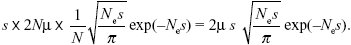
See Figure P22.6.
|
| ii) |
The peak is at s = 0.0375. Differentiating the formula with respect to s and setting it to zero shows that, in general, the maximum rate is contributed by changes of effect 3/(2Ne). Typically, this implies weak selection and rather slow evolution of isolation by this mechanism of random drift in small demes. NOTE 22L
|
|
Answer 22.7
|
| i) |
An AQ allele has a chance pB of being paired with BP allele, in which case it gains fitness 1 + s; otherwise, it has the baseline fitness of 1. Thus, its average fitness is WAQ = 1 + spB. An AP allele has a fitness 1 + s if it is paired with a BQ allele, but zero otherwise. Therefore, its average fitness is WAP = (1 + s)qB. The selection coefficient is WAP – WAQ = (1 + s)qB – (1 + spB) = s(qB – pB) – pB. The same formulae hold for alleles BP, BQ, with A and B swapped.
|
| ii) |
The change in allele frequency due to selection is given exactly by
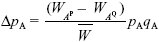
(see Box 28.1). However, the rate of migration is low, and so we expect the frequency of BP to be low: it is incompatible with the most common allele at A. Therefore, we can take  ~ 1, qB ~ 1, and WAP – WAQ ~ (s – pB); both s and pB will be small. Adding the effects of gene flow from a population with pA = 0 (Box 16.1): ~ 1, qB ~ 1, and WAP – WAQ ~ (s – pB); both s and pB will be small. Adding the effects of gene flow from a population with pA = 0 (Box 16.1):
ΔpA ~ (s – pB)pAqA + m(0 – pA) = (s – pB)pAqA – mpA.
Similarly for the other gene, with gene flow from a population with pB = 1,
ΔpB ~(s – pA)pBqB + m(1 – pB) = (s – pA)pBqB + mqB.
|
| iii) |
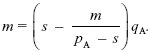
At equilibrium, AP might be lost (pA = 0) and/or BQ might be lost (qB = 0). If neither of these happen, we can cancel pA from the equation for ΔpA = 0, and qB from the equation for ΔpB = 0. This gives an equilibrium with both polymorphic loci:
0 = (s – pB)qA – m,
0 = (s – pA)pB + m.
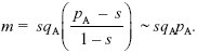
Since AP is common, pA > s, and we can solve the second equation to give pB = m/(pA – s). Substituting into the first equation,
This can be solved graphically (Fig. P22.7) or using the formula for a quadratic equation. It is convenient to rearrange the formula to keep all the terms with m on one side:
For migration rate m = 0.002, the solution is pA = 0.278 (the leftmost point where the blue curve crosses the lower red line in Fig. P22.7). There is another equilibrium at pA = 0.712, which is unstable: For pA lower than this, allele frequency falls toward the lower stable equilibrium at pA = 0.278, and above this, it increases to fix AP. For the higher rate of m = 0.0035, there is no polymorphic equilibrium: Gene flow swamps divergence (see Fig. P22.8).
|
| iv) |
The threshold rate of gene flow is where the migration rate touches the maximum of the blue curve in Figure P22.7: m* = s/4. NOTE 22M
|
|
Answer 22.8
|
| i) |
2Nm = 2 × 104 × 10–6 = 0.02 genes are introduced every generation. Each has a chance ~2s = 0.1 of getting established and fixing. Therefore, the rate of successful migration is 4Nms = 0.002 per generation. It will take on average 500 generations for the allele to be successfully transmitted between the two populations. NOTE 22N
|
| ii) |
On average, it takes 1/4Nms = 500 generations for the new allele to invade the second deme. During this time, we expect 500Λ = 10 substitutions to occur at other loci, and there is a chance of 500Λp = 0.01 that one of these will be incompatible with the new allele, so that it remains confined to the population in which it arose.
|
| iii) |
The chance is just k × p.
|
| iv) |
The rate at which new alleles successfully establish in one of the populations is 2Λ. The chance that they will remain confined to their original population is kp (the chance that one of the k existing differences is incompatible) plus Λp/4Nms (the chance that a new incompatibility arises before the allele can spread). Thus,
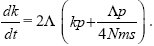
This can be integrated using the method of Box 28.3:
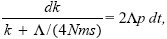
so
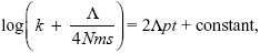
with k = 0 at t = 0. Therefore, the constant is log(Λ/4Nms), and we rearrange to find
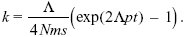
With the parameters given, it will take about 115,000 generations for 100 incompatibilities to arise. Over this time, the total number of substitutions would be 2Λt = 4600. In the absence of gene flow, the number of incompatibilities that would have arisen is (Λt)2p = 5290. Thus, gene flow slows down divergence, but does not prevent it altogether. See Figure P22.9.
|
| v) |
Differences in environment could greatly accelerate divergence in the early stages: Selection for different alleles in different populations could establish differences, and, later, alleles incompatible with these could arise even with no help from environmental differences. Reduced recombination could also encourage divergence by reducing the effective rate of gene flow: Alleles could not recombine onto the opposite genetic background so quickly (see pp. 647–648). NOTE 22O
|
References
Kondrashov A.S. 2002. Accumulation of Dobzhansky–Muller incompatibilities within a spatially structured population. Evolution 57: 151–153.
Lande R. 1979. Effective deme sizes during long-term evolution estimated from rates of chromosomal rearrangement. Evolution 33: 234–251.
Navarro A. and Barton N.H. 2002. Accumulating postzygotic isolation genes in parapatry: A new twist on chromosomal speciation. Evolution 57: 447–459.
Turelli M. and Orr H.A. 1995. The dominance theory of Haldane’s Rule. Genetics 140: 389–402.
Turelli M. and Orr H.A. 2000. Dominance, epistasis and the genetics of postzygotic isolation. Genetics 154: 1663–1679.
Walsh J.B. 1982. Rate of accumulation of reproductive isolation by chromosome rearrangements. Am. Nat. 120: 510–532.
Wright S. 1941. On the probability of fixation of reciprocal translocations. Am. Nat. 75: 513–522.
|