Oscillations in Abundance of Predators and Prey

The abundance of species may oscillate in a regular way, which cannot be explained by external factors such as the weather. One of the best-known examples is of the abundance of hare and lynx in the Canadian Arctic, whose fluctuations are documented over many years in records from trappers collected by the Hudson’s Bay Company (Fig. WN28.1). Qualitatively, such oscillations can be explained by the coupling between predator and prey: As prey increase, so do predators, which then reduce prey numbers; as their prey dwindle, predators decline, completing the cycle. However, such interactions do not always lead to stable oscillations. A mathematical model is needed to show under just what conditions oscillations will occur.

A simple and widely used model of ecological interactions was proposed independently by Lotka and Volterra in the 1920s. Let n₁ be the number of prey and n₂ the number of predators. We suppose that the rates of change are

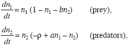
where a,b,ρ > 0. The terms in parentheses are the fitnesses of prey and predators, respectively. At low density, prey numbers grow at rate 1, but predators decline at rate –ρ, because they have no prey. As the number of prey, n₁, increases, the fitness of prey declines as a result of intraspecies competition, but the fitness of the predators increases. As the number of predators, n₂, increases, the fitness of both prey and predators declines.

We have chosen to make some of the coefficients 1, leaving only three parameters: a, the effects of prey on predator fitness; b, the effects of predators on prey fitness; and ρ, the rate of decline of predators in the absence of prey. The model is in fact quite general. We have chosen to scale time so as to make the growth rate of prey at low density 1, and we have measured population sizes in units such that the effects of each species on its own fitness appears as 1. For more on how to simplify equations by rescaling them, see Otto and Day (2007, Chapters 8 and 9).

We can understand the behavior of this simple system by seeing that prey increase whenever 1 – n₁ – bn₂ > 0 and that predators increase whenever –ρ + an₁ – n₂ > 0. These two relationships define two lines, which are shown in Figure WN28.2. Below the short dashed line (1 – n₁ – bn₂ = 0), prey increase, indicated by a yellow tint; to the right of the long dashed line (–ρ + an₁ – n₂ = 0), predators increase (red tint). Thus, the ecosystem evolves along trajectories indicated by the four arrows: prey increase and predators decrease when both are rare (bottom left), and so on. Where the two lines meet, there is an equilibrium. There is also an equilibrium where only prey are present (n₁ = 1, n₂ = 0, bottom right).

It is not obvious whether these two equilibria are stable or unstable. First, we can ask whether predators can increase from low density, when prey are at equilibrium with n₁ = 1. The predators’ rate of increase will then be (a – ρ), and so they can invade provided a > ρ. To find whether predators can coexist with prey, we must find whether the internal equilibrium is stable. Let this equilibrium be at n₁^*, n₂^* and consider small deviations, so that n₁ = n₁^* + ε₁, n₂^* + ε₂. Discarding terms involving ε₂, we have a pair of linear equations that describe the system near to equilibrium:

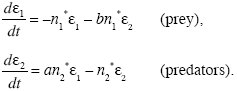
As in the previous example (Box 28.3), we seek solutions that grow or shrink steadily, as exp(λt). However, in the example of Figure WN28.2, there is no solution of this form: no real value of λ satisfies the equations above when we substitute ε₁ = e₁exp(λt), ε₂ = e₂exp(λt). In cases such as this, there will be a solution of the form ε₁ = e₁exp(λt)sin(ωt), ε₂ = e₂exp(λt)sin(ωt + θ), which correspond to oscillations in numbers. In this example, λ = –0.64, and so the equilibrium is stable. The two species coexist, but when perturbed away from equilibrium, numbers fluctuate up and down as they settle back (Fig. WN28.2B). For more on limit cycles, see Otto and Day (2007, Chapters 8 and 9).

In this model, coexistence is stable for any positive values of a, b, and ρ, provided a > ρ so that predators can invade from low density. We will now look at a slightly different model, in which there is no stable equilibrium:

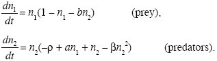
The growth of the prey is described by the same equation. However, the growth rate of the predators now increases with increasing predator density (+n₂ term in the second equation); this is known as an Allee effect, in which reproduction increases with increasing density. This might be, for example, because it is easier to find a mate when the population is denser. Predator fitness then decreases again as predators become yet more abundant (βn₂²), which prevents their fitness increasing indefinitely.

The dynamics are qualitatively similar, with the two lines of zero predator fitness and zero prey fitness, marking out four regions in which the ecosystem evolves in different directions (arrows in Fig. WN28.3A). As before, predators can invade provided a > ρ, and there is then an internal equilibrium where the two lines cross. Slight perturbations away from this equilibrium again oscillate but now grow at a rate λ = 0.10. Thus, there is no stable equilibrium. Instead, the abundance of predator and prey oscillates in a stable limit cycle (Fig. WN28.3B). Although the linear stability analysis does not prove that this will be the outcome, the presence of an unstable equilibrium, from which fluctuations oscillate with ever-increasing magnitude, suggests that a limit cycle will be reached.