Evolution Chapter 18 Answers
|
Answer 18.1
|
| i) |
The variance in allele frequency increases as vpq/N in a haploid population of N genes, where v is the variance in offspring number. (The formula on p. 419 is for a diploid population, which contains 2N genes, and for which the variance in allele frequency increases as vpq/2N.) For a Poisson distribution of offspring number with mean 1, v = 1, and so Ne = N. In this example, the variance of offspring number is v = 1/2, and so Ne = 2N.
|
| ii) |
Now the mean fitness is 1.02, and so the allele increases at a rate s = 0.02 from low frequency.
|
| iii) |
It is simplest to work out the probability of loss, Q (see Chapter 28). If one copy of the allele produces no offspring, then it is certain to be lost; if it produces one, it has chance Q of being lost; and if it produces two, then there is a chance Q2 that both will be lost. So, Q = 0.24 × 1 + –0.5 × Q + 0.26 × Q2. This has the (nontrivial) solution Q = 0.923, and so the probability of fixation is P = 1 – Q = 0.077.
|
| iv) |
The approximation 2s(Ne/N) gives 2 × 0.02 × 2 = 0.08, which is close to the exact solution.
|
| v) |
The chance that n copies will all be lost is Qn, and so the chance that one at least will fix is 1 – Qn. (See Fig. P18.2.)
|
|
Answer 18.2
|
| i) |
The expected time to the common ancestor of a pair of genes is 2Ne = 2 × 10⁶ generations, and so they will be separated by, on average, 4 × 10⁶ generations of divergence. The expected number of mutations that will occur during this time is only θ = 4Neμ = 3 × 10–9 × 4 × 106 = 0.012 (see p. 426). Thus, we can assume that any one codon will usually be fixed for one of the four possibilities. NOTE 18C
|
| ii) |
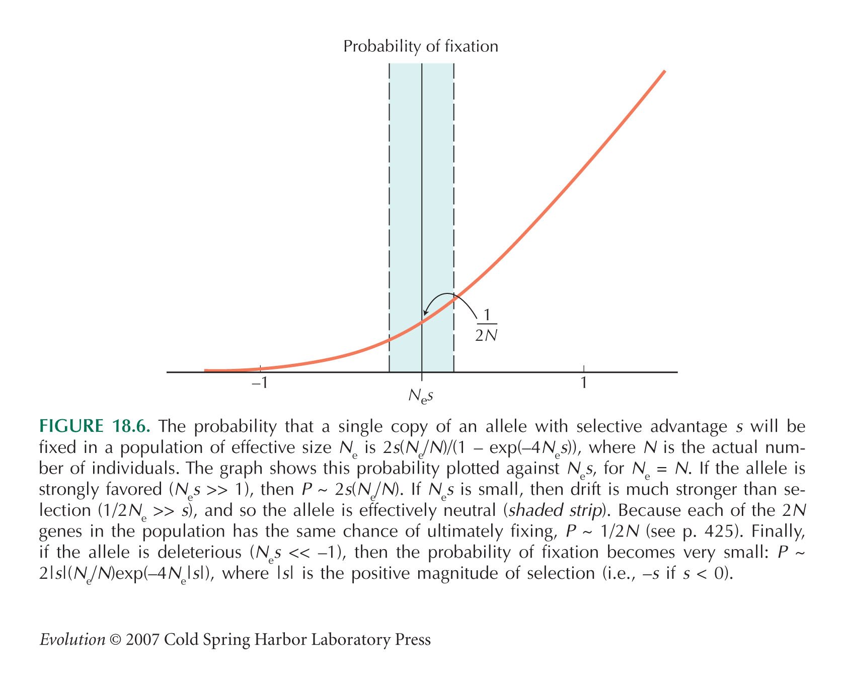
The probability of fixation of a single mutation is P = 2s(Ne/N)/(1 – exp(–4Nes)) (see Fig. 18.6). For s = +10–6, this is P+ ~ 2s = 2.0 × 10⁻⁶, whereas for s = –10–6, this is P– = 3.7 × 10⁻⁸. (Assume that Ne = N.)
|
| iii) |
At equilibrium, the rate of shifts from GUU must equal the rate of shifts to GUU. All mutations from GUU change to one of the other three codons, whereas only one-third of mutations from any of the other three go to GUU. If the proportion of codons that are GUU is x, then we have 2N × μ/3 × P+ (1 – x) = 2N × μ × P– × x, and so x = 0.948. Note that this frequency is independent of the number of mutations per generation, Nμ, which just determines the (very slow) rate at which equilibrium is approached. Cancelling 2 Nμ, and cancelling 2|s|(Ne/N) from the formula in Figure 18.6, we have
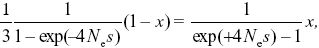
and so x/(1 – x) = (1/3)exp(4Nes). Now,  = (1 + s)2, and so the relative frequencies of the two kinds of codons are proportional to 2Ne = exp(4Nes), as given by Wright’s formula (Eq. 18.1), and to the relative rates of mutation to and from the two kinds (1/3). = (1 + s)2, and so the relative frequencies of the two kinds of codons are proportional to 2Ne = exp(4Nes), as given by Wright’s formula (Eq. 18.1), and to the relative rates of mutation to and from the two kinds (1/3).
|
| iv) |
If we see a ratio of 70/30 = (1/3)exp(4Nes) then we can infer that Nes = (1/4)loge(7) = 0.49, implying that s = 5 × 10⁻⁷. NOTE 18D
|
|
Answer 18.3
|
| i) |
Generalizing the calculation at the end of Box 18.1, we have a rate of decline in fitness of 2 × f × U × s × (P/P0). Here, f is the fraction of mutations that have effect Nes, U is the total mutation rate per genome, and P/P0 = 4Nes/(exp(4Nes) – 1) is the probability of fixation P divided by the probability for a neutral allele, 1/2N. (Here, we focus on deleterious alleles, and so substitute –s for s in the formula of Fig. 18.6.) We can write the selection coefficient as s = Nes/Ne. Thus, the rate of decline is (2fU/Ne)(Nes)(4Nes/(1 – exp(–4Nes)).) (See Fig. P18.3.) Mutations with effect Nes in the range 0.1–1.5 contribute most to the decline.
|
| ii) |
If deleterious mutations have been fixed at a site, then once Ne increases again, the chance that the original favorable allele will fix is approximately 2s(Ne/N). There are 2Nμ mutations per generation in total, and so the rate at which they accumulate is 4Nesμ. This is the product of the rate of mutation to the specific favorable allele, μ, and 4Nes, the strength of selection relative to drift. Even if 4Nes is large (~103, say), per-site mutation rates are so low (~10–9 per year, say) that it will take a very long time for fitness to recover.
|
|
Answer 18.4
|
| i) |
In each generation, additive variance is reduced by VA/2Ne as a result of random drift (see p. 418). Balancing this against the increase VM due to mutation, we have VA = 2NeVM = VE. Therefore, we expect a heritability of 50%. (See also Problem 15.4.) NOTE 18E
|
| ii) |
The question gives a selection gradient β = 0.1/ . Hence, R = VAβ = 0.1 per generation (from Eq. 17.3). . Hence, R = VAβ = 0.1 per generation (from Eq. 17.3).
|
| iii) |
Each diploid locus contributes a variance 2μα2 = 2 × 10–5 × 0.52VE = 0.5 × 10⁻⁵VE. Since VM = 0.005VE, we must have n = 1000 loci influencing the trait. NOTE 18F
|
| iv) |
Each allele increases the trait value by α = ±0.5 ; half of these have a negative effect and so cannot fix in a large population, but the other half increase relative fitness by +αβ = 0.05. (See the answer to Problem 17.12.) The probability of fixation of such alleles is approximately 2s = 0.1. NOTE 18G
|
| v) |
Summing over n = 1000 loci, in every generation, 2nNeμ/2 = 2 × 1000 × 100 × 10–5/2 = 1 favorable mutations are produced, and 2snNeμ = 0.1 actually fix. NOTE 18H Finally, the effect of each substitution is to increase the trait by 2α = . We therefore expect R = 0.1 per generation, just as we obtained using the argument based solely on phenotype. NOTE 18I
|
|
Answer 18.5
|
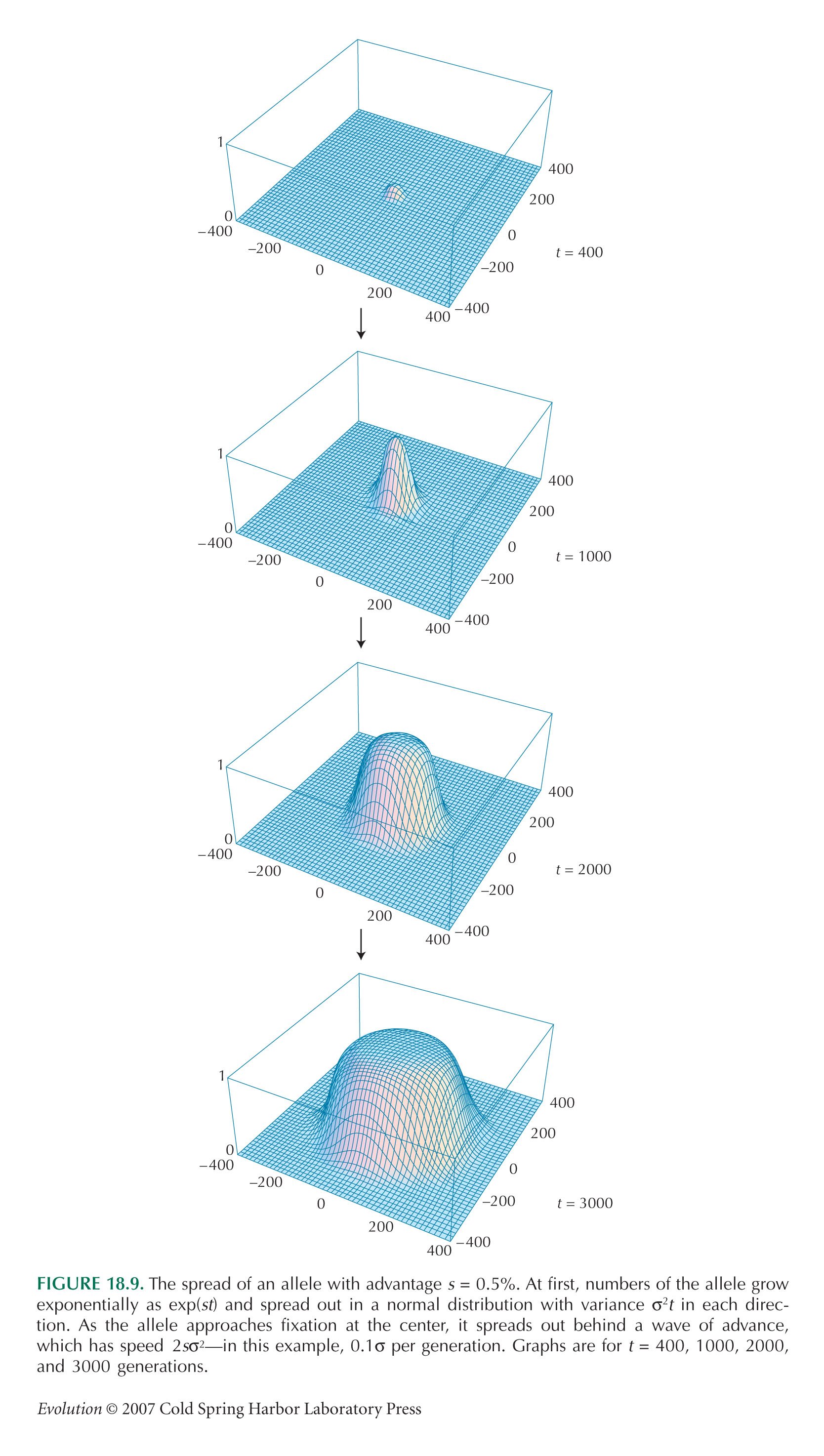
| i) |
The initial frequency is p0 = 1/2N = 10–8, and so the simplest deterministic prediction would be that p = p0(1 + s)t ~p0 exp(st) initially. As the allele becomes common, it must approach fixation at a maximum frequency of 1. This is enough to sketch the graph (see Fig. P18.4): On a log scale, it will be a straight line up to when p ~ 1, after which it flattens out. For a more accurate answer, we know from Eq. 17.2 that
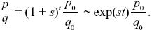
Therefore NOTE 18J
|
| ii) |
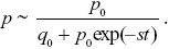
The number of copies of the allele in the population is approximately exp(st); this is not altered by the movements of individuals in space. NOTE 18K We also know that the distribution spreads out in a normal distribution with variance σ2t. Therefore, the density of copies of the allele distance x from the point of origin is
The allele frequency is the density of copies divided by the total population density, 2N/R2, where R = 1000 km is the range. So, we have allele frequency
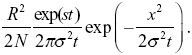
This equals 0.5 at x = 0 at t ~ 600 generations.
|
| iii) |
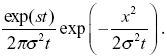
Once the allele has spread to high frequency, it expands behind a wavefront that advances with speed c =  (see Fig. 18.9). The area within this wavefront is A = πr2 = πc2t2, and so the frequency of the allele is A/R2 = π2σ2st2/R2, where t is now the time elapsed since the allele became common. (see Fig. 18.9). The area within this wavefront is A = πr2 = πc2t2, and so the frequency of the allele is A/R2 = π2σ2st2/R2, where t is now the time elapsed since the allele became common.
|
| iv) |
If we suppose that the wavefront starts to spread steadily when the allele frequency at the origin gets to p = 0.5, we get the picture in Figure P18.5.
The frequency increases exponentially at first, but then slows drastically to increase as ~t2, because natural selection is only effective at the narrow interface between populations fixed for alternate alleles. Figure P18.5 shows two approximations, one accurate when the allele is rare everywhere (left) and the other when it has become common (right).
|
| v) |
The second phase will last until the new allele has reached the edges and traveled about 600 km. (If the habitat is square, there are 500 km from center to the nearest edge, but 700 km to the corner.) Thus, we have 600 km =  t, and so t = 3000 generations. This compares with about 430 generations for the first phase: Exponential growth is much faster than steady spread through a large habitat. t, and so t = 3000 generations. This compares with about 430 generations for the first phase: Exponential growth is much faster than steady spread through a large habitat.
|
|
Answer 18.6
|
| i) |
On either side, the most common chromosome arrangement will be favored, because it is less often found in the less-fit heterozygotes. Selection alone would maintain a sharp boundary between populations fixed at frequencies 0 or 1. However, gene flow (σ2) blurs this boundary, leading to a smooth cline (as, e.g., in Fig. 18.16).
|
| ii) |
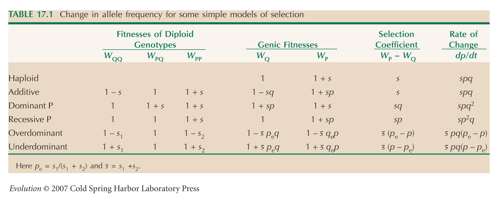
We approximate gene flow by diffusion, and selection as being continuous in time. Table 17.1 gives the fitnesses of the three genotypes as 1 + s1:1:1 + s2, and the rate of change of allele frequency as dp/dt = (s1 + s2)pq(p – pe), where pe = 1/2 and s1 = s2 = s. The diffusion approximation is given by the equation at the end of Box 28.6, with no mean displacement (M = 0) and variance V = σ2. So,
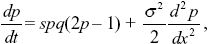
where q = 1 – p.
|
| iii) |
At equilibrium, dp/dt = 0. Substituting for p shows that p = 1/(1 + exp(–a x)) is a solution, with a2 = 2s/σ2.
|
| iv) |
The maximum gradient in allele frequency is at x = 0, p = 1/2 is dp/dx = a/4. If the width w is defined as the inverse of this, then w =  . .
|
|
Answer 18.7
|
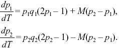
| i) |
Assuming that selection is weak, we can approximate the rate of change of allele frequency in the two demes as
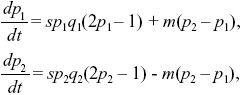
where qi = 1 – pi. We can simplify by dividing both sides by s and scaling time as T = st. Then, the solution depends only on the ratio between migration and selection, M = m/s:
|
| ii) |
Trivially, there are stable equilibria where the same arrangement is fixed in both demes (p1, p2 = 0 and p1, p2 = 1; blue disks at bottom left and top right of Fig. P18.6), and there is an unstable equilibrium at the center, with equal frequencies in each deme (p1 = p2 = 1/2). With no gene flow, different chromosome arrangements can fix in the two demes, and we expect that with low enough gene flow, similar asymmetrical equilibria will still exist and be stable. Above a critical rate of gene flow, however, one or other arrangement will fix in both demes.
Because the model is symmetrical, we expect the same amount of polymorphism in each deme; that is, we look for an equilibrium with p1 = q2, p2 = q1. Setting the two equations above to zero, and making this substitution, both reduce to 0 = p2q2(p2 – q2) – M(p2 – q2).
We are not interested in the symmetrical equilibrium at p2 = q2 = 1/2 and so we can cancel (p2 – q2) to find that p1q1 = p2q2 = M = m/s. This corresponds to two possible equilibria (p1 low, p2 = q1 high, and vice versa). Because pq cannot be larger than 1/4, we see that this equilibrium exists when M ≤ 1/4.
|
| iii) |
To determine whether the equilibria are stable, we set p1 =  + ε1, p2 = + ε1, p2 =  + ε2, and ignore small terms such as ε12. ( = + ε2, and ignore small terms such as ε12. ( =  denote the equilibrium frequencies, with denote the equilibrium frequencies, with  = M.) Substituting p = p* + ε in pq(p – q) gives approximately ε(6pq – 1) = ε(6M – 1). Thus, = M.) Substituting p = p* + ε in pq(p – q) gives approximately ε(6pq – 1) = ε(6M – 1). Thus,
In general, we can find whether the ε1, ε2 grow or shrink by looking for solutions that change steadily, with ε1, ε2 both proportional to exp(λt). There will be two solutions: The λ with the largest magnitude corresponds to the solution that grows fastest and is called the leading eigenvalue (Box 28.3). In this case, a simpler trick can be used. If we add up the equations, the last terms cancel, and we have d(ε1 + ε2)/dt = (6M – 1)(ε1 + ε2). Therefore, if M < 1/6, the deviation of the total allele frequency from equilibrium shrinks. This determines the threshold for stability.
We see that for 1/6 < M < 1/4, the asymmetrical equilibria exist, but are unstable. For 1/4 < M, these equilibria do not even exist. Figure P18.6 shows how allele frequencies in the two demes evolve, for M just below or just above the threshold at 1/6. NOTE 18L
|
|
Answer 18.8
|
| i) |
Homozygotes are impossible, and PQ heterozygotes cannot be fertilized by pollen carrying either allele.
|
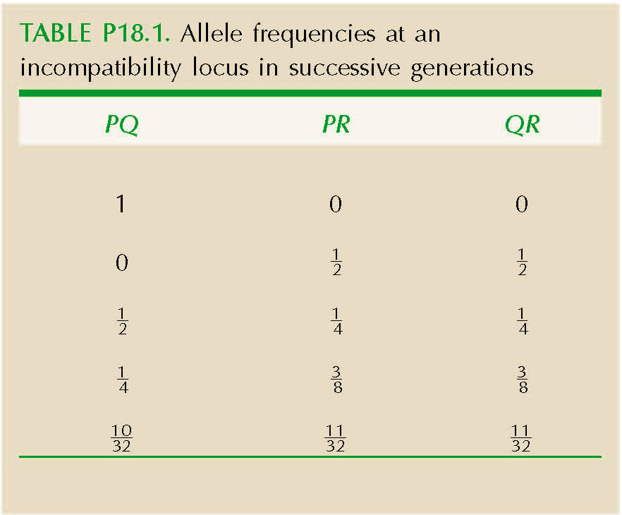
| ii) |
Call the alleles P, Q, R. Only the heterozygotes PQ, PR, QR can be produced; these must be fertilized by R, Q, P pollen, respectively. Thus, a PQ plant produces equal proportions of PR and QR, and similarly for the others. The genotype frequencies therefore rapidly approach equality (see Table P18.1 and Fig. P18.7).
|
| iii) |
At equilibrium, the three alleles, and the three heterozygous genotypes, are equally frequent. Any genotype of pollen can only fertilize one-third of ovules that do not carry their allele, a reduction in relative fitness by two-thirds. Because one-half of fitness comes from female function and one-half from male, the average fitness is reduced by one-third overall. (We assume that females produce the same number of offspring—variation in fitness is due to differences in the success of male gametes.)
|
| iv) |
A fourth allele can fertilize all the existing genotypes, and so has fitness 1 via both male and female. Overall, its fitness is 1, compared with the fitnesses of the three existing alleles, 2/3.
|
| v) |
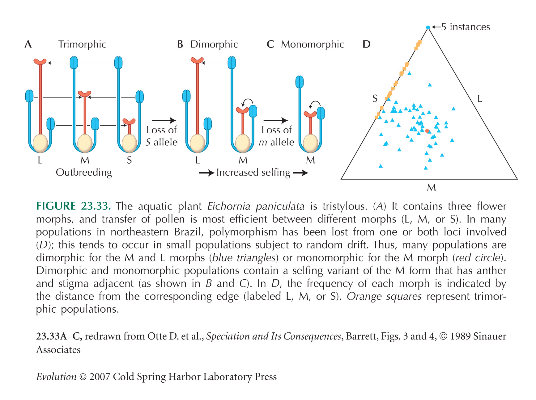
This analysis suggests that an infinite number of incompatibility alleles could invade. However, rare alleles may be lost by chance (see, e.g. Fig. 23.33): A population of N diploid individuals will carry many fewer than the maximum possible of 2N alleles. In addition, there may be constraints on how many incompatibility alleles can be produced, depending on how many functional sequences can be produced by the genes involved.
|
|
Answer 18.9
|
| i) |
With hard selection, the contribution that each allele makes to the next generation (i.e., its fitness) is simply the arithmetic average over A and B: WP = (0.9 + 0.45)/2 = 0.675, WQ = (0.3 + 0.9)/2 = 0.6. Therefore, at low frequency P increases relative to Q at a rate (WP/WQ) = (0.675/0.6) = 1.12; when Q is rare, it increases by a ratio (WQ/WP) = 0.89. It is impossible for both to be maintained as a polymorphism.
|
| ii) |
First, think about how fast P increases from some low frequency, p. Within patch A, allele P increases by a ratio 0.9/0.3 = 3, and within patch B, decreases by 0.45/0.9 = 1/2. Since each patch contributes a fixed fraction (here, 1/2), the frequency overall increases by (1/2)(3 + 1/2) = 1.75. Similarly, Q will increase from low frequency by a ratio (1/2)(1/3 + 2) = 1.167. Because both P and Q can invade there, a stable polymorphism can be maintained (i.e., there is a protected polymorphism). NOTE 18M
|
| iii) |
Arguing in the same way, but allowing for contributions 1 – α:α from the two patches rather than 1/2:1/2, we find that the rate of increase of P is 3(1 – α) + (1/2) α, and of Q is (1/3)(1 – α) + 2α. These are both greater than 1, allowing polymorphism, in the range 0.4 < α < 0.8. See Figure P18.8.
|
| iv) |
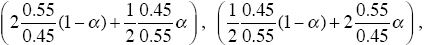
We now have rates of increase of P of
and of Q of
This allows polymorphism in the range 0.45 < α < 0.55. When selection is weak, polymorphism is only possible in a very narrow parameter range in this model.
|
| v) |
Now, two-thirds of the P alleles start in patch B and one-third start in patch A, and conversely for allele Q. If allele P is at frequency p in the population as a whole, then P and Q alleles enter patch A in proportions (2/3)p:(1/3)q and into patch B in the ratio (1/3)p:(2/3)q. When P is rare, therefore, its initial frequency within A is 2p and within B is (1/2)p; similarly for Q. The rates of increase of P and Q from low frequencies are therefore now
respectively, and polymorphism is possible in the range 0.29 < α < 0.71. When alleles systematically tend to exploit different habitats, polymorphism becomes possible for a much wider range of parameters. In fact, even if the alleles have the same survival within patches, habitat preference will maintain polymorphism. What matters is that the alleles tend to be in different patches, so that when they are rare, they experience less competition and gain a frequency-dependent fitness advantage. NOTE 18N
|
|
Answer 18.10
|
| i) |
The frequency of a recessive lethal at equilibrium is p =  . (Set the selection coefficient to s = 1 in Box 18.2.) Therefore, the incidence of the disease is equal to the mutation rate: p2 = 1/90,000 = 1.11 × 10⁻⁵. . (Set the selection coefficient to s = 1 in Box 18.2.) Therefore, the incidence of the disease is equal to the mutation rate: p2 = 1/90,000 = 1.11 × 10⁻⁵.
|
| ii) |
Assume that most of the deleterious alleles are eliminated in heterozygotes, so that (following Box 18.2) p = μ/hs, with hs = 0.02. Assuming Hardy–Weinberg proportions, p2 = 1/90,000, and so p = 1/300. Therefore, μ = hsp = 6.67 × 10⁻⁵. As a check on the assumption, the proportion of deaths as heterozygotes is 2pqhs ~ 13.3 × 10⁻⁵, and as homozygotes is p2 = 1.1 × 10⁻⁵. So, ignoring the latter should not be a bad approximation.
A more accurate calculation would follow the genotypes through one generation. The frequency of the Q allele after selection is
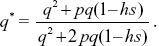
A fraction (1 – μ) of Q alleles remain as Q after mutation, and so, at equilibrium,
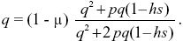
When the proportions of selective deaths and mutations are small (p2,hsp,μ << 1), this simplifies to p2 + hsp ~ μ, which just balances the loss of alleles through selective deaths against the increase due to mutation. The solution for hs = 0.02, p2 = 1/90,000 is μ = 7.77 × 10⁻⁵, somewhat greater than the estimate of 6.67 × 10⁻⁵ made ignoring the deaths of homozygotes.
|
| iii) |
With inbreeding, the incidence of the disease is (1 – F)p2 + Fp: in a fraction F of individuals, the two genes are identical by descent, and so the chance of being homozygous for the disease allele is p, not p2. If most deaths are in inbred marriages (i.e., (1 – F)p2 << Fp), then Fp = 1/90,000 and so we estimate p = 22.2 × 10⁻⁵. In both cases i) and ii), the loss of heterozygotes (2hsp) is much smaller than the loss of homozygotes (~Fp) and so we estimate μ = Fp, and μ = 1.11 × 10⁻⁵, as in i). NOTE 18O
|
|
Answer 18.11
|
| i) |
For small deviations, fitness is approximately 1 – (z – zopt)2/2Vs. To find the selection coefficient, think about the average trait value of the two alternative alleles (see pp. 388–392). If the mean is at the optimum, and the allele is rare, then the common wild-type allele will have fitness close to 1, and the alternative rare allele will have fitness reduced by α2/(2Vs). With α = 0.2 and Vs = 20VE, we have a selection coefficient of 0.001.
|
| ii) |
The total mutation rate over the diploid genome is U = 2nμ = 0.02. In every generation, mutation generates alleles at frequency μ at each gene and effect α, and so the increase in variance due to mutation at a single gene copy is μα2. Summing over the 2n genes in a diploid gives Vm = 2nμα2. So, the mutational heritability is VM/VE = 2nμα2/VE = Uα2/VE = 0.02 × 0.04 = 0.0008.
|
| iii) |
At each locus, a mutation/selection balance maintains allele frequency p = μ/s = 10–5/10–3 = 0.01. Therefore, the genetic variance maintained in total, over the 2n genes in a diploid individual, is VG = 2nα2pq = 2000 0.04 0.01 × 0.99 ~ 0.8VE. The heritability is h2 = VG/(VG + VE) = 0.44.
|
| iv) |
In general, VG = 2Σi αi2 pi qi, and we know that in a mutation-selection balance, pi qi = μi/si. Therefore, VG = 2Σi αi2(μi/si) = 2Σi αi2(2Vsμi/αi2) = 2UVs (assuming that pi << 1). This is independent of the effects of individual alleles or the mutation rate to each allele. All that matters is the total mutation rate, U, and the strength of selection, 1/Vs. NOTE 18P
|
| v) |
If we assume that mutations affect these traits in the same way (i.e., with α = 0.2 ), then the selection coefficient arising from effects on 20 traits will be 20 times that on one trait, or 0.001 × 20 = 0.02. Thus, the allele frequencies and the genetic variance that is maintained will be 20 times smaller. Allowing for the effects of pleiotropy makes it much harder to explain high heritabilities.
|
| vi) |
If we just set the selection coefficient to = 0.01, we find that VG = 2nα2μ/ = VM/ = 0.0008VE/0.01 = 0.08VE, a much lower heritability. = VM/ = 0.0008VE/0.01 = 0.08VE, a much lower heritability.
|
|
Answer 18.12
|
| i) |
To find the equilibrium, we must balance the increased numbers of alleles due to mutation against the loss due to selection against heterozygotes, and against homozygotes: μ = (hsp + sp2). With random mating, most loss of fitness is due to heterozygotes, rather than homozygotes. Therefore, the last term sp2 is negligible relative to hsp, and so we find the standard formula for the allele frequency μ/hs = 10–5/0.01 = 0.001. (This is consistent, because the loss of fitness in heterozygotes is 2hspq ~ 2 × 10⁻⁵, whereas that in homozygotes is only sp2 = 10–7.)
The mean fitness at each locus is therefore (1 – 2hspq) = (1 – 2μ). (Note that this is independent of selection at each locus; see p. 552.) Multiplying over n = 10,000 genes, we have a total reduction of (1 – 2μ)n ~ exp(–2nμ) = 0.82.
|
| ii) |
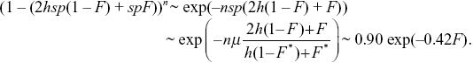
An inbred individual has probability 1 – F of having a genotype in Hardy–Weinberg proportions and hence has mean fitness 1 – 2μ, as in i). It has probability F of being homozygous, and so having mean fitness 1 – sp = 1 – sμ/hs = 1 – 10μ. Overall, the mean fitness is

This is proportional to exp(–BF) with B = 0.8; B is a standard measure of the strength of inbreeding depression. B can be measured by plotting the log of fitness against F and measuring the scope.
|
| iii) |
Balancing the increased numbers of alleles due to mutation against the loss due to selection against heterozygotes and against homozygotes, we have μ = (1 – F*)(hsp + sp2) + F*sp, where F* = 0.1 is the average inbreeding coefficient across all the individuals in the population. The first term gives the loss of alleles in the fraction 1 – F of outbred individuals: The term sp2 is negligible as before, and so we can write μ = (1 – F)hsp + Fsp, giving p = μ/((1 –F*)hs + F*s) = 10–5/(0.9 × 0.01 + 0.1 × 0.1) = 0.00053. The fitness of an individual with inbreeding coefficient F is
Thus, the strength of inbreeding depression has decreased by about one-half, from B = 0.8 to B = 0.42, because partly recessive alleles are exposed to selection in heterozygotes, and so are eliminated.
|
| iv) |
At each of the ten genes, heterozygote advantage maintains polymorphism with equal allele frequencies. The chance of being homozygous is 1/2 if the individual’s genes are not IBD, and 1 if they are IBD. Homozygotes have fitness reduced by 10% and so the average reduction in fitness of an individual is 0.1((1 – F)/2 + F) = 0.05 + 0.05F. Multiplying over the ten genes, we have fitness (1 – 0.05 – 0.05F)10 ~ 0.60 exp(–0.5F). Thus, balancing selection at a few loci can produce comparable amounts of inbreeding depression to mutation at many loci.
|
| v) |
It is not easy to distinguish the causes of inbreeding depression: If deleterious recessives are tightly linked, and in repulsion (i.e., +–/–+), then they will behave like overdominant alleles at a single locus. However, one simple prediction is that continued inbreeding will “purge” deleterious recessives, so that if these are responsible for inbreeding depression, then the strength of inbreeding depression will decrease (as in iii)). That is not the case for overdominant alleles (as in iv)).
|
References
Clayton G.A. and Robertson A. 1955. Mutation and quantitative variation. Am. Nat. 89: 151–158.
Hill W.G. 1982. Predictions of response to artificial selection from new mutations. Genet. Res. 40: 255–278.
Karlin S. and McGregor J. 1972. Application of method of small parameters to multi-niche population genetics models. Theor. Pop. Biol. 3: 180–209.
Robertson A. 1960. A theory of limits in artificial selection. Proc. R. Soc. Lond. B 153: 234–249.
|


