Evolution Chapter 19 Answers
|
Answer 19.1
|
| i) |
The mean frequency was initially 0.1, and it is now 0.199. The variance across the ten replicates is estimated as 0.0021, and the variance of the mean of the ten is estimated as 1/10 of this. Thus, the standard deviation of the mean is  = 0.014, and the change in allele frequency is 0.099/0.014 ~ 7.1 s.d. A change as large or larger than this is very unlikely to arise by chance. NOTE 19M = 0.014, and the change in allele frequency is 0.099/0.014 ~ 7.1 s.d. A change as large or larger than this is very unlikely to arise by chance. NOTE 19M
|
| ii) |
On average, the ratio of allele frequencies has changed by a factor (p20/q20) (q0/p0) = 2.24 over 20 generations. This equals (WP/WQ)20. Therefore, we estimate WP/WQ = 2.241/20 = 1.041, or a selection coefficient of 4.1%.
|
| iii) |
A selection coefficient of 4.1% corresponds to 6.9 standard deviations. A change of approximately 2 standard deviations would be judged significant, and so a selection coefficient of 4.1 × 2/6.9 = 1.2% should be just detectable. NOTE 19N
|
| iv) |
The variance between cages is estimated as 0.0021. From the binomial distribution (Box 28.5), the variance due to sampling 400 genes is expected to be pq/400 = 0.199 × 0.801/400 = 0.00040, which is much smaller. The excess variance, 0.0017, is due to 20 generations of random drift, and (from Box 15.1), it is expected to be pq(1 – (1 – 1/2Ne)20), where p, q are the average allele frequencies. NOTE 19O For Ne >> 20, this is very close to ~20pq/2Ne. Substituting in p = 0.199, q = 0.801, and solving, we find that Ne ~ 940. Twenty generations of random drift in a population of Ne ~ 1000 produces about four times as much variation as sampling 200 individuals from each cage at the end.
|
| v) |
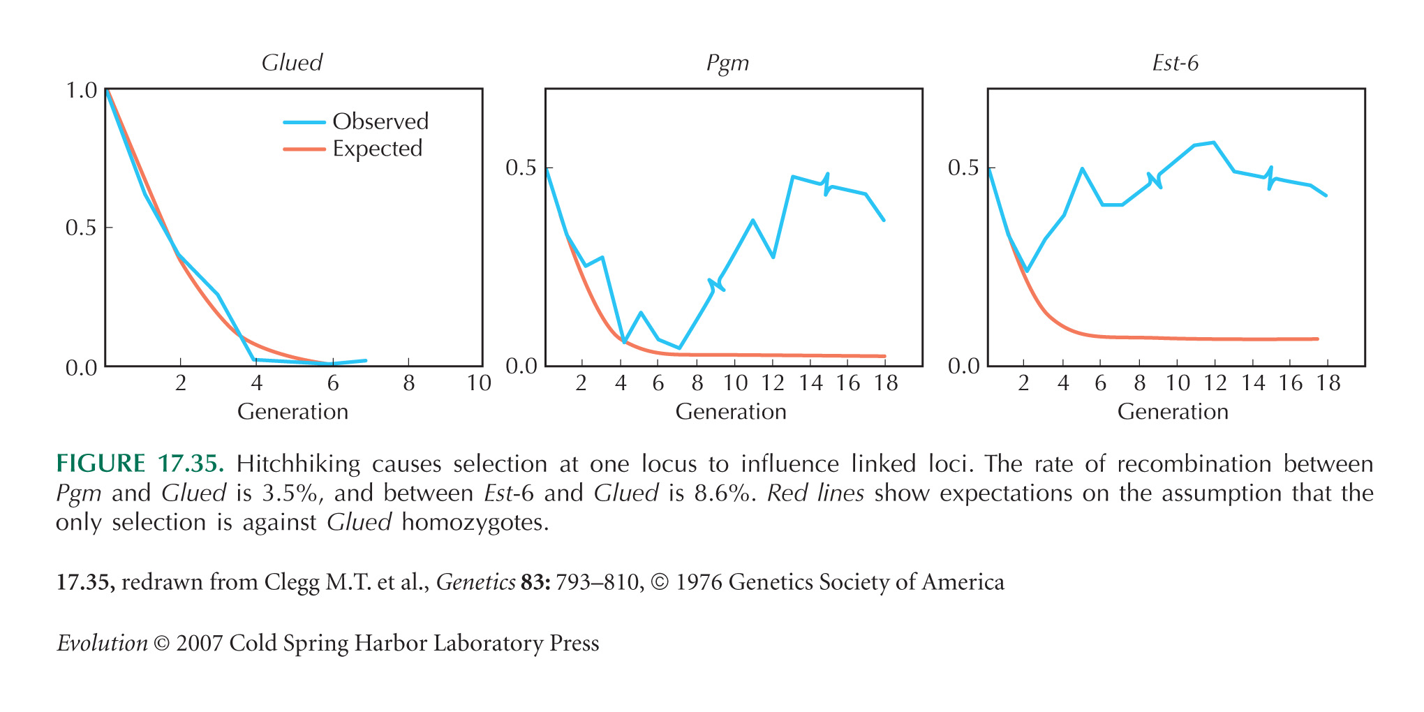
The same pattern of change could be produced if the observed allele is very tightly linked to another allele that has selective advantage 4.1%. Eventually, however, the alleles would be separated by recombination, and so the observed allele frequency would stop increasing if the observed allele were itself neutral. (See next question.) Thus, the experiment could be run for longer.
The observed allele could also be separated from its genetic background by backcrossing for many generations into a standard population, so as to produce a nearly isogenic line.
Another possibility would be to change the environment in a way that is expected to alter selection on the observed enzyme alleles (e.g., adding ethanol in a study of alcohol dehydrogenase).
The ideal experiment would be to use genetic manipulation to produce two genotypes that differ only at the site of interest. This requires considerably more effort, however, even in D. melanogaster.
|
|
Answer 19.2
|
| i) |
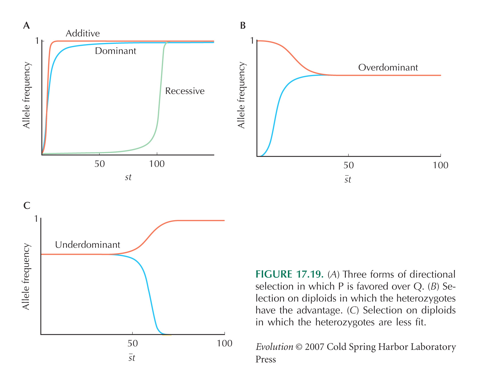
There is a rapid decline in the frequency of the F allele, followed by a slower increase, and finally an approach to an apparent equilibrium at a frequency of about 0.4. A plausible explanation is that the two parent populations differed not just for the F/S alleles, but also for at least one other locus, tightly linked to Adh. If it is initially associated with a strongly deleterious allele, it will fall quickly, until it recombines away. After the initial association has broken down (after ten generations, say), the allele will increase as a result of its own effects on fitness. If heterozygotes are fittest, or there is some kind of negative frequency-dependent selection, then it will approach an equilibrium (see Fig. 17.19B). NOTE 19P
This qualitative explanation can be made at least roughly quantitative. Over the 15 generations from generations 10 to 25, the allele increases from p = 0.05 to 0.26. Since the ratio (p/q) changes by a factor WP/WQ in each generation, we know that
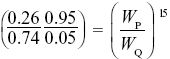
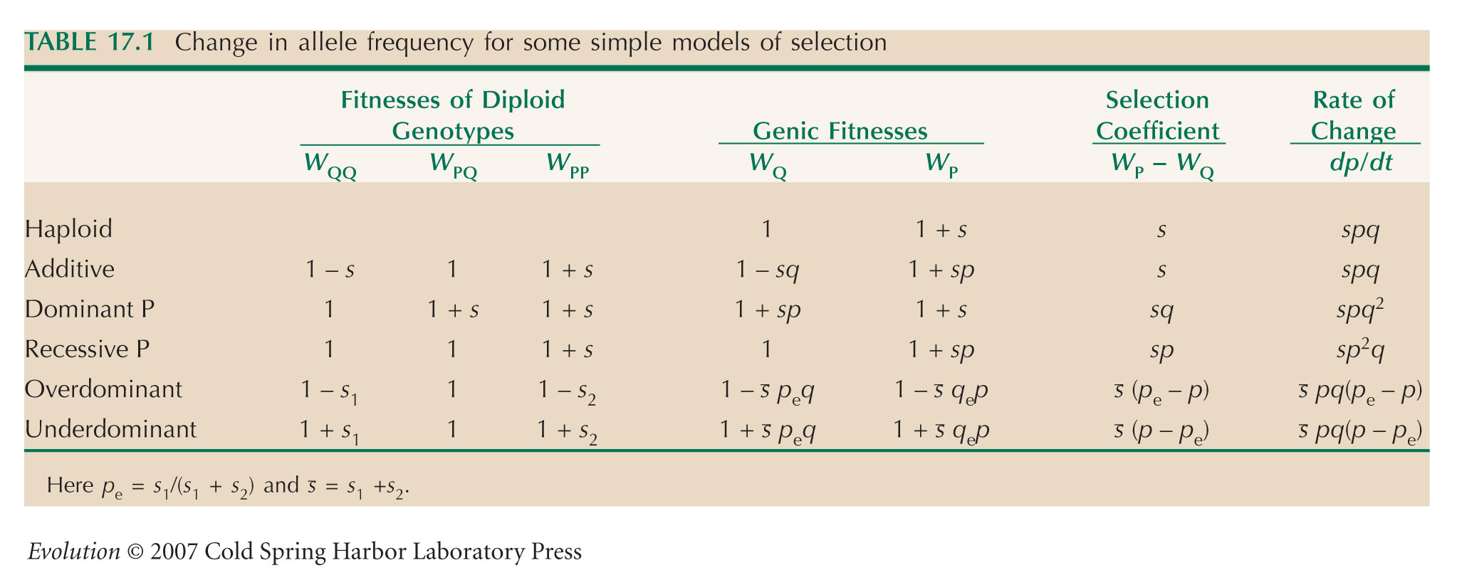
and so WP/WQ = 1.135; that is, the selective advantage of P when increasing from low frequency is about 0.135. The mean allele frequency during the last 50 generations is 0.39, giving an estimate of the equilibrium frequency. From Table 17.1, if the fitnesses of SS, SF, FF are 1 – s1, 1, 1 – s2, then we have equilibrium at s1/(s1 + s2) = 0.39, and rate of increase from low frequency of F given by selection coefficient s1 = 0.135. Therefore, s2 = 0.21. Frequency-dependent selection could also account for the stable polymorphism.
In the first five generations, the frequency falls from 0.5 to 0.095, and so we estimate WP/WQ = 0.717. If the effects of the alleles at the linked loci multiply, then the effect of the linked locus itself (after dividing by the effect of the observed locus) is 0.717/1.135 = 0.632. It would be possible to estimate the recombination rate between the two loci from the time taken for associations to disappear (about ten generations). To do that, we would fit a model with two linked loci, under selection in opposite directions. However, the rough calculations outlined here give reasonably accurate estimates. NOTE 19Q
|
| ii) |
The main flaw in the design is that the population starts as an F1 between two divergent populations, so that there is absolute linkage disequilibrium between every variant that differs between the populations. (This was done deliberately in the experiment of Fig. 17.35, for example.) Therefore, there will inevitably be strong hitchhiking effects. These linkage disequilibria do dissipate eventually, and so simply running longer experiments will give more confidence that changes are eventually due to selection on the locus itself. Alternatively, one could start by backcrossing for t generations into the parental population that carries S, selecting for the F allele in each generation. This will generate a nearly isogenic line that carries a block of material from the F population around the F allele itself; this block will be of map length ~1/t. A simpler alternative is to start with individuals drawn from a large outbred population, hoping that it is close to linkage equilibrium. Ideally, however, one would use genetic manipulation to generate populations that differed only at the site of interest.
The experiment could also use replicate cages, with several replicates starting from each of several base population crosses. This would allow effects of initial genetic background to be separated from subsequent random fluctuations.
|
|
Answer 19.3
|
| i) |
Male survivors are slightly larger (by 0.27 mm) and less variable (variances 0.403 vs. 0.288). The difference in mean length is just significant (P = 4% on a t-test), whereas the difference in variance is not significant on an F-test. Female survivors have almost the same mean but are significantly less variable on an F-test (0.173 vs. 0.434; P = 3.2%). Thus, there is directional selection on males for increased humerus length and stabilizing selection on females for reduced variability in humerus length. (See Fig. P19.4.)
|
| ii) |
We can think about the consequences of directional and stabilizing selection separately. The selection differential on male humerus length is the difference between the mean after selection and the mean before: Sm = 18.77 – (18.77 × 51 + 18.50 × 36)/87 = 0.11 mm. (For comparison, the phenotypic standard deviation in the original population was  = 0.58 mm.) The overall selection differential, S, is the average of that in males and in females. Since directional selection on females was weak, we can take S = Sm/2 = 0.055 mm. If humerus length has high heritability (as is usually the case), we expect that a large fraction of this selection differential will be transmitted as a response to selection: R = h2S. With h2 ~ 1, it would take about ten episodes of selection for the mean to change by one phenotypic standard deviation. = 0.58 mm.) The overall selection differential, S, is the average of that in males and in females. Since directional selection on females was weak, we can take S = Sm/2 = 0.055 mm. If humerus length has high heritability (as is usually the case), we expect that a large fraction of this selection differential will be transmitted as a response to selection: R = h2S. With h2 ~ 1, it would take about ten episodes of selection for the mean to change by one phenotypic standard deviation.
The consequences of stabilizing selection are much harder to predict, because they depend on the genetic basis of trait variation (pp. 482–484). The snowstorm led to a reduction in variance by a factor of 0.288/((51 × 0.288 + 36 × 0.403)/87) = 0.858 in males and by 0.537 in females. However, this will be replenished by recombination, by segregation of alleles in heterozygotes, and by mutation, in ways that cannot be predicted without knowing a great deal about the nature of the genetic variation. It remains very hard to explain the existence of high levels of trait variation despite observations of strong stabilizing selection such as this (see pp. 513–515).
As in many other studies, Bumpus’ data show differences in selection on males and on females. The consequences depend on whether variation in the two sexes is due to the same genes or to different genes. At one extreme, the same alleles might be responsible for trait variation in the two sexes. Then, the effect of selection just depends on its average over the two sexes. On the other hand, the traits could in principle be genetically independent. It is best to view “male humerus length” and “female humerus length” as two separate traits that may be genetically correlated (see p. 457) to some degree.
|
|
Answer 19.4
|
| i) |
Assuming Hardy–Weinberg proportions, the frequencies of alleles cr and sd can be estimated as the square root of the frequency of the corresponding homozygote. The frequency of allele d can be found directly as the sum of the frequency of dd homozygotes plus half the frequency of Dd heterozygotes. NOTE 19R These are shown in Figure P19.5.
|
| ii) |
Drawing straight lines through the central region by eye and estimating cline width as in Figure P19.3 gives estimates of w ~ 17.7, 17.3, 13.1 km for cr, sd, d, respectively.
|
| iii) |
Using the formula w =  gives estimates of selection on these three loci of 0.072, 0.075, 0.130. NOTE 19S gives estimates of selection on these three loci of 0.072, 0.075, 0.130. NOTE 19S
|
|
Answer 19.5
|
| i) |
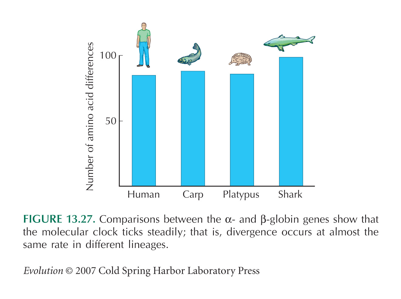
It is extraordinary that the amount of divergence is so similar across such different pairs of vertebrate species. Each pair does share some early ancestry (when the α and β globins had just diverged in the primordial vertebrate), but the genes have spent most of their divergence in different lineages, and much of it in very different kinds of organisms (see Fig. 13.27).
|
| ii) |
The chance of no change over the two lineages that trace back to the common ancestor, T = 500 × 106 years ago, is (1 – λ)2T ~ exp(–2λT). (Recall that the two lineages have been diverging for a total of 2T generations.)
|
| iii) |
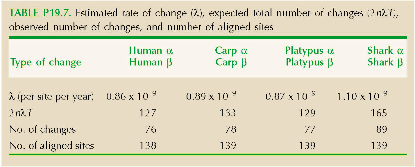
We can equate this to the fraction of sites that have not changed, Q. (The chance that a site would change, and then change back to the same amino acid, is negligible.) Thus, we set Q = exp(–2λT), and so λ = –loge(Q)/(2T). The total number of substitutions over n sites is estimated as 2λTn. (See Table P19.7.)
|
| iv) |
The number of substitutions follows a Poisson distribution with expectation 2λT at each site. So, the chance of there having been exactly one substitution at a site is 2λT exp(–2λT), and the expected number across all sites is n times this.
|
| v) |
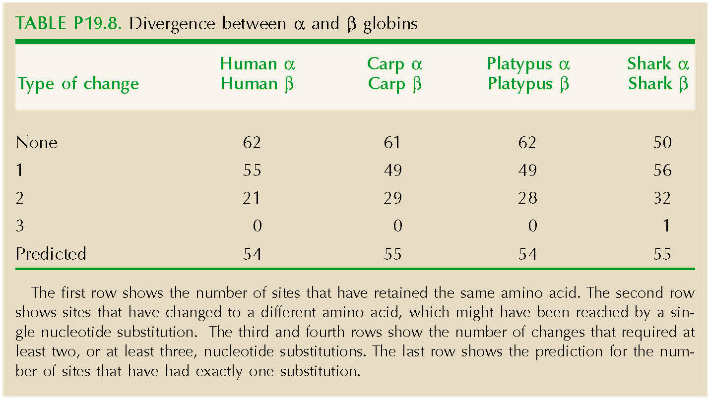
The genetic code constrains which amino acids can be reached by a single base change (Fig. P19.6). For example, asparagine can change to serine by a single change at the second position (e.g., AAC→AGC). However, a change from asparagine to proline requires at least two base changes (e.g., AAC→CAC→CCC). Table P19.8 shows the number of sites that have retained the same amino acid. The second row shows sites that have changed to a different amino acid, which might have been reached by a single nucleotide substitution. The third and fourth rows show the number of changes that required at least two, or at least three, nucleotide substitutions. The last row shows the prediction for the number of sites that have had exactly one substitution, 2nλT exp(–2λT), which is quite close.
|
|
Answer 19.6
|
| i) |
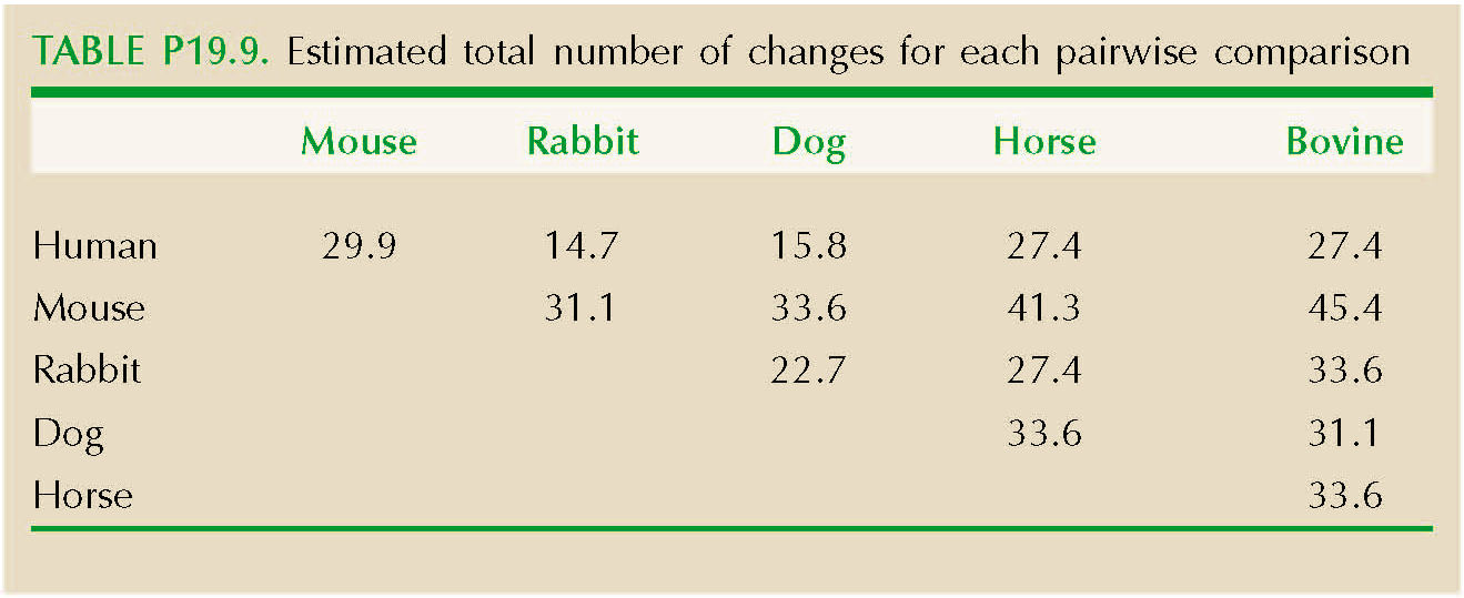
There are 27 differences between the β globins of human and mouse out of 146 amino acid sites. If the rate of divergence per site, per year, is λ, then the chance of a substitution over 2T generations of divergence is 2λT, The chance that there will be no change is Q = exp(–2λT), and so we can estimate the expected number of changes over n sites as –n loge(Q)—here, 29.9 changes. Using the same method for all 15 comparisons, we get the results shown in Table P19.9.
|
| ii) |
The variance and mean of these differences, corrected for multiple substitutions, are 61.8 and 29.9, respectively. If the number of species were very large, we could use their ratio directly to estimate the variance/mean ratio of the underlying rates, xi: this gives R = var(dij)/mean(dij) = 61.8/29.9 = 2.1. However, var(dij) = (2(n – 2)/n)var(xi) and mean(dij) = 2mean(xi). Therefore, we estimate R = var(xi)/mean(xi) = (n/(n – 2))var(dij)/mean(dij) = 2.1 × 6/4 = 3.1. NOTE 19T NOTE 19U
|
| iii) |
The variance in numbers of substitutions is estimated to be about three times larger than expected from a Poisson distribution. This may well reflect real variation in the rate of molecular evolution (see p. 531); for example, substitutions might occur in bursts, as proteins adapt to a changed environment. Rates might also vary because of differences in generation time or degree of selective constraint between lineages. However, the variance may also exceed the mean because of errors in the correction for multiple substitutions, or because the phylogeny is not in fact a star. Then, the variability in numbers of differences would reflect variation in degree of relationship, rather than in the rate of molecular evolution. (See Web Notes.)
|
|
Answer 19.7
|
| i) |
The allele frequencies are {8/12, 2/12, 1/12, 1/12}. The proportion of homozygotes that we expect with random mating is the sum of squares of these frequencies, or 0.486.
|
| ii) |
The probability of seeing k = 4 alleles is
105258076θ4/θ (θ + 1)(θ + 2)···(θ + 11)
(see Fig. P19.7).
|
| iii) |
The most likely estimate is θ = 4Neμ = 1.67. We expect homozygosity 1/(1 + θ) = 0.374, which is lower than seen in the sample.
|
| iv) |
The probability of seeing as much homozygosity as this, or more, is the probability of seeing this configuration, {8,2,1,1}, or a more homozygous one. The only configuration of four alleles that would be more homozygous is {9,1,1,1}: All others have more genetic variation. So, the probability is
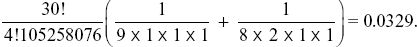
So, this configuration is unusually homozygous—the chance that we would see a configuration as homozygous as this, or more so, is only 0.0329. In other words, it has more rare alleles than expected.
|
|
Answer 19.8
|
| i) |
The ratio Pn/Ps averages  = 0.223. Assuming neutrality, this is an estimate of the ratio between the rate of neutral mutations that alter amino acid sequence (i.e., nonsynonymous mutations) and the rate of neutral synonymous mutations (Dn/Ds). If Dn/Ds = Pn/Ps, then we predict that the nonsynonymous divergence due to random drift should be Dn* = Ds(), as shown below. = 0.223. Assuming neutrality, this is an estimate of the ratio between the rate of neutral mutations that alter amino acid sequence (i.e., nonsynonymous mutations) and the rate of neutral synonymous mutations (Dn/Ds). If Dn/Ds = Pn/Ps, then we predict that the nonsynonymous divergence due to random drift should be Dn* = Ds(), as shown below.
|
| ii) |
The difference between the observed and the expected nonsynonymous divergence, Dn – Dn*, can be attributed to positive selection. The proportion of positively selected substitutions can therefore be estimated as α = 1 – Dn*/Dn. The average is best estimated as 1 –  / / , where an overbar indicates an average over genes. Thus, we estimate the average fraction of positively selected substitutions as , where an overbar indicates an average over genes. Thus, we estimate the average fraction of positively selected substitutions as  = 0.45. NOTE 19V (See Table P19.10.) = 0.45. NOTE 19V (See Table P19.10.)
|
| iii) |
The strength of this test is that synonymous and nonsynonymous variation should be affected in the same way by population history (e.g., population bottlenecks), as long as both are neutral. This makes the test robust to population structure. Deviations from Dn/Ds = Pn/Ps could arise from various kinds of selection:
Some of the nonsynonymous polymorphism may consist of slightly deleterious mutations, which would never get to high frequency and contribute to Dn. That would bias the predicted Dn* upward—the opposite to the observed pattern. Balancing selection on nonsynonymous polymorphism would make the predicted Dn* higher—again, the opposite of the pattern seen.
So, the excess divergence at nonsynonymous sites is strong evidence that selection is responsible for a substantial fraction of amino acid substitutions.
|
|
Answer 19.9
|
| i) |
Nucleotide diversity is reduced over about 50 kb (see the black line in Fig. P19.8).
|
| ii) |
The ratio of allele frequencies must increase from p/q ~ 1/2N to ~1. We know from Equation 17.2 that this ratio increases as (1 + s)t ~ exp(sT), and so we have that 2N = exp(sT). Therefore, T ~ (1/s)loge(2N) (see p. 469). NOTE 19W
|
| iii) |
As the genome carrying the new mutation increases from low frequency, it will recombine with other genomes in every generation, until by the time it reaches fixation, only a small fragment of the original genome remains, surrounding the favorable mutation itself. If we focus on a site that recombines at rate c, the chance that no recombination occurs in any of the T generations is (1 – c)T ~ exp(–cT).
|
| iv) |
The nucleotide diversity is defined as the chance that the two randomly chosen genes carry different bases at a site. If one or both of the chosen genes trace back via a recombination event to some random gene in the ancestral population, then the chance that they are different is just the same as anywhere in the genome (π0 say). However, if both trace back, with no recombination, to the single original genome that carried the favorable mutation, then they are identical by descent. Assuming that the sweep is recent, they must then be identical and contribute zero diversity. The chance that neither of the two lineages experience a recombination is exp(–cT)2 = exp(–2cT). So, we have π = π0(1 – exp(–2cT)).
|
| v) |
If diversity is reduced for about 25 kb on either side of the selected locus, this corresponds to c = 25,000 × 1.5 × 10–8 = 3.75 × 10⁻⁴. Setting 2cT = 1 as the region over which diversity is substantially reduced, and using T = (1/s)log(2N) with N = 106, we get s ~ 0.01. The curve shown in Figure P19.8 roughly fits the πs, averaged over the three species (black line); it assumes π0 ~ 0.035 and s = 0.01.
|
|
Answer 19.10
|
| i) |
From Figure 19.21A, diversity seems to be reduced by exp(–1) ~ 0.37 when the rate of recombination is about c = 0.5 cM per megabase, or 0.5 × 10⁻⁸ Morgans per base pair. So we can set 1 = U/R = 2μL/cL = 2μ/c, where the genome length L cancels, and μ is the rate of deleterious mutation per base pair per generation. (The factor 2 arises because U is defined as the total mutation rate per diploid genome.) Thus, we estimate that μ = 2.5 × 10⁻⁹ per base pair per generation. (See Fig. P19.9.)
|
| ii) |
The total rate of mutation in Drosophila is estimated as 3 × 10⁻⁹ per base pair per generation (see p. 426). So, most mutations must be deleterious if background selection is to explain reduced diversity in regions of reduced recombination. This seems implausible, given that most of the Drosophila genome does not code for protein and is not strongly conserved between species. NOTE 19X
The true causes of the pattern shown in Figure 19.21A remain unknown: One possibility is frequent selective sweeps.
|
|
Answer 19.11
|
| i) |
A fraction 0.32 of pairs of genes will both be linked to the rarer allele. These will be drawn as if from a pool of size 0.3N, where N is the overall population size. Therefore, nucleotide diversity will be reduced to 0.02 × 0.3. Similarly, a fraction 0.72 of genes will have diversity reduced to 0.02 × 0.7. However, a fraction 2 × 0.3 × 0.7 will be linked to different alleles, and we know that these alleles have been maintained in the population for a very long time. Therefore, the linked sites will be completely divergent and under the infinite-sites model will have π = 1. NOTE 19Y Overall, then, diversity is increased to π = 0.02(0.32 + 0.72) + 2 × 0.3 × 0.7 = 0.43.
|
| ii) |
A fraction 0.72 = 0.49 of pairs of lineages is linked to the more common allele, and so coalesced 105 generations ago. (We ignore the possibility of coalescence more recently than 105 generations ago.) So, the nucleotide diversity is the expected number of substitutions per base pair, over 2 × 10⁵ generations of divergence, or 2Tμ = 0.001. The remaining pairs will coalesce within the ancestral population and so will have the usual π = 0.02 typical of the genome as a whole. Overall, then, diversity is reduced to 0.51 × 0.02 + 0.49 × 0.001 ~ 0.011. Because one of the alleles arose recently, the effect is that of a selective sweep, not a long-term balanced polymorphism (see p. 542).
|
|
Answer 19.12
|
| i) |
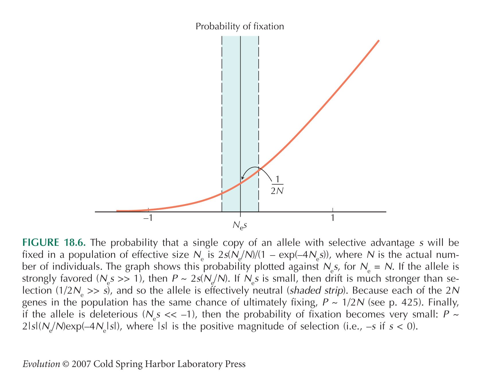
The probability of fixation of a mutation that reduces fitness by s is (from the formula in Fig. 18.6) 2(Ne/N)s/(exp(4Nes) – 1). There are 2Nμ mutations at each site, and there are two sites that can be disrupted within each pair, giving a net rate of fixation of 8Nesμ/(exp(4Nes) – 1) per pair per generation.
|
| ii) |
We know from i) the rate of substitutions that disrupt pairing. Relatively soon after a pair is disrupted, it will either be restored, or will change to a new, stable pair. So, a simple argument is that the net rate of change to a new stable pair is half the rate calculated in i), 4Nesμ/(exp(4Nes) – 1). This is the rate at which both sites in the pair change and should be compared with the rate of change per site under neutral evolution, μ. The observed reduction in rate is 0.021/0.044; setting this equal to 4Nes/(exp(4Nes) – 1) implies Nes = 0.665.
|
| iii) |
The rate at which the site that mutated will mutate back to its original state is μ/3; at the same rate, the other site in the pair will mutate to produce a new pair. For example, GC could mutate to GA, and then either mutate back to GC, or mutate to TA. (Note that any base can mutate to three other bases, only one of which may restore pairing. We assume that mutation to each is equally likely.) The probability that any mutation that restores pairing will be fixed is 2(Ne/N)s/(1 – exp(–4Nes)), and so the rate of substitutions that produce a different pair is 2N × (μ/3) × 2(Ne/N)s/(1 – exp(–4Nes)) = (μ/3)4Nes/(1 – exp(–4Nes)). The rate of return to the original pair is the same. Both rates are faster than the rate of disruptive substitutions by a factor (1/6)exp(4Nes).
|
| iv) |
The ratio between the rate of production of mispaired sites, to the rate of restoration of pairing, is 1:(1/3)exp(4Nes) = 1:4.77. Therefore, the fraction of mispaired sites is expected to be 1/(1 + 4.77) = 0.17. NOTE 19Z NOTE 19AA This can be understood if Nes is large. Then, it is very unlikely that two compensatory mutations at unlinked sites could ever fix, because the population has to pass through an “adaptive valley” of reduced mean fitness. However, substitutions are possible with tight linkage. Mispaired sites will be maintained at a frequency of μ/s per site, and so at a rate μ2/3s, the compensatory mutation will arise. If there is no recombination, these will stay together, and can drift to fixation with probability 1/2N. The decrease in rate of molecular evolution with map distance is hard to reconcile with the argument above that Nes is not very large.
|
|
Answer 19.13
|
| i) |
The ratio of fitnesses between the two extremes is (1.01)1000 ~ exp(10) ~ 22,000. The ratio between fitnesses of an average individual (with 500 heterozygous loci) and the maximum possible is 1.01500 = 148. It does not seem plausible that the average fitness could be so far below what is possible—remember that the fitness of an individual is defined as the number of offspring.
|
| ii) |
The mean and variance of the number of heterozygous loci in an individual are 500 and 250, respectively.
|
| iii) |
95% of the population is expected to lie within ±2 standard deviations (i.e., with between 468 and 532 loci, or relative fitnesses of 0.73 to 1.37). This range is not unreasonable. Thus, moderately strong selection can act on many polymorphisms, but we cannot suppose that their fitness effects just multiply together: This would imply that a completely heterozygous individual would have absurdly high fitness. Rather, fitness must increase at a diminishing rate as the number of heterozygous loci increases, so that it never becomes absurdly high. This implies a certain kind of epistasis (p. 552).
|
|
Answer 19.14
|
| i) |
The maximum possible fitness is 1, compared with a mean fitness of 1 – 2s(q2) – s(2pq) = 1 – 2sq(p + q) = 1 – 2sq. So, the loss of mean fitness caused by the presence of Q is 2sq. To see this more directly, each copy of allele Q reduces fitness by s, and there are on average 2q per individual.
|
| ii) |
The total substitution load is
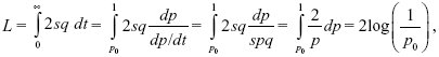
as calculated by Haldane (1957). Here, we have changed from thinking of the load 2sq as a function of time to thinking of it as a function of allele frequency (i.e., Fig. P19.10B, rather than P19.10A). (See Box 28.2.)
|
| iii) |
The same method gives a load sq2 per generation, and a total load of
which is half as great. This is because the dominant allele increases faster from low frequency. Conversely, the load due to a strictly recessive allele is much greater, because it takes such a long time to rise from low frequency.
|
|
Answer 19.15
|
| i) |
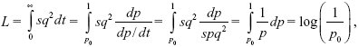
From Box 28.1, dp/dt = spq. This has a solution t = (1/s) log((pt/qt)(q0p0)) (Box 28.2), where allele frequencies change from p0, q0 to pt, qt over t generations. In this example, the initial allele frequency is p0 = 1/2N, and q0 ~ 1. So, we can rearrange the solution as (pt/qt) = (1/2N)exp(st). (This can also be derived from Eq. 17.2 by setting (WP/WQ)t = (1 + s)2 ~ exp(st). The allele frequency at time t is pt ~ exp(st)/(2N + exp(st)).)
|
| ii) |
In the first generation, there is a single genome carrying AUBP and so uP = 1. All the other genomes carry BQ, and so uQ is very close to the initial overall frequency of the neutral allele, u0 = 0.2. NOTE 19BB
|
| iii) |
Because selection does not act directly on AU, AV, their frequencies within the two alternative genetic backgrounds, uP, uQ, stay the same. So, as p changes to p*, the overall allele frequency changes from u to u* = p*uP + q*uQ, and the change in allele frequency is Δu = u* – u = Δp(uP – uQ). In continuous time, du/dt = (dp/dt)(uP – uQ). Crucially, recombination does not change allele frequencies, but only shuffles the combinations of alleles. So, this simple argument applies to the whole generation, including both selection and recombination.
|
| iv) |
At meiosis, a genome carrying BP may meet another genome carrying BP, in which case recombination will not make any difference. If BP meets a BQ allele, however, there is a chance c that a recombination event will bring an A allele that was associated with BQ into coupling with BP. The probability of a change is therefore c × q, and if there is a change, uP will change to uQ. Therefore, uP changes to uP(1 – cq) + uQcq, and similarly, uQ changes to uQ(1 – cp) + uPcp. The difference (uP – uQ) changes to (uP – uQ)(1 – c), and so over t generations, uP – uQ decreases by a factor (1 – c)t ~ exp(–ct). Since uP – uQ is initially (1 – u0), it will be (1 – u0)exp(–ct) at time t.
|
| v) |
The rate of change in u is just (uP – uQ) times the rate of change of p. Now, allele BP sweeps to fixation relatively quickly, at about (1/s)log(2N) generations: Most of the time is spent getting from one copy up to appreciable frequency. So, the total change in u will equal the value of (uP – uQ) at this time (Δu ~ (uP – uQ)Δp, and Δp ~1). So, Δu ~ Δu0exp(–c/s)log(2N) = u0(2N)–c/s = 0.149. (An exact calculation gives Δu = 0.153 [see Fig. P19.11].)
|
| vi) |
The chance that the mutation BP first arose with AU is u0, and leads to an increase of +(1 – u0)(2N)–c/s. The chance that it arose instead with AV is 1 – u0 and would lead to a decrease of –u0(2N)–c/s. Overall, then, the mean change is zero, and the variance of the change in allele frequency (i.e., the mean square deviation) is u0(1 – u0)(2N)–2c/s.
|
| vii) |
The rate of increase of the variance in neutral allele frequency (in effect, the rate of random drift) is Λu0(1 – u0)(2N)–2c/s. However, we must average the recombination rate over random positions of mutations on the genetic map. These can be uniformly distributed between 0 and R/2, assuming that the neutral gene is in the middle of the genetic map. So, the average is
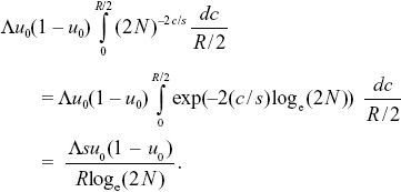
If we define the effective population size by setting this rate of random drift to u0(1 – u0)/2Ne, we have 2Ne = (R/Λs) loge(2N). For the parameters given here, 2Ne = 168,000. This depends only weakly on population size, through loge(2N), and is proportional to the density of selective sweeps per map length (Λ/s) times the selection coefficient. NOTE 19CC NOTE 19DD (See Fig. P19.11.)
|
References
Gillespie J.H. 2000. Genetic drift in an infinite population: The pseudohitchhiking model. Genetics 155: 909–919.
Gillespie J.H. 2000. The neutral theory in an infinite population. Gene 261: 11–18.
Haldane J.B.S. 1957. The cost of natural selection. J. Genet. 55: 511–524.
Stephan W. 1996. The rate of compensatory evolution. Genetics 144: 419–426.
Stephan W.S. and Kirby D.A. 1993. RNA folding in Drosophila shows a distance effect for compensatory mutations. Genetics 135: 97–103.
|


